Project page

TimeOmni-o1: Bidirectionally Coupling Time Series Foundation Models and LLMs for Multimodal Reasoning and Forecasting

Ziyang Zhang^1,2, Shenyi Li², Wen Wu², Chao Zhang^1,2†

¹Tsinghua University ²Shanghai Artificial Intelligence Laboratory ^†Corresponding author

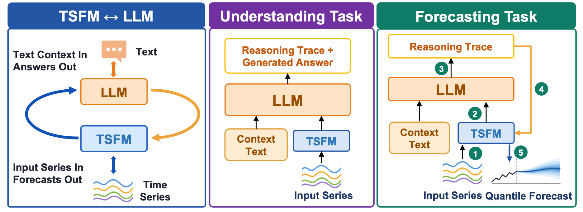
We present TimeOmni-o1, which couples a pretrained TSFM and an LLM bidirectionally. In one direction, the TSFM encodes the series in compressed form for the LLM, which reasons over it together with the text. In the other, the LLM’s reasoning is fed back into the TSFM, which produces the forecast conditioned on it.

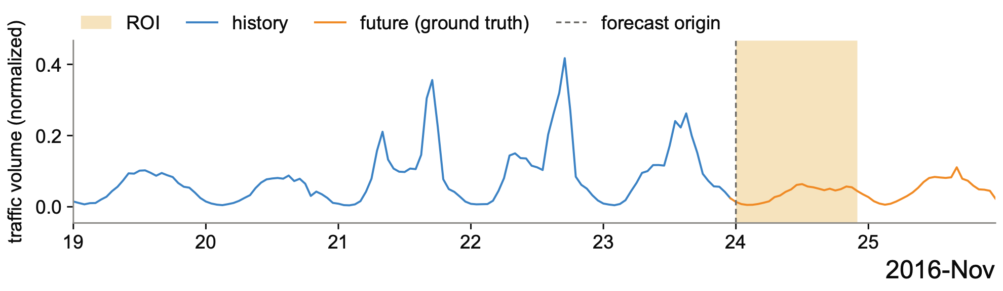
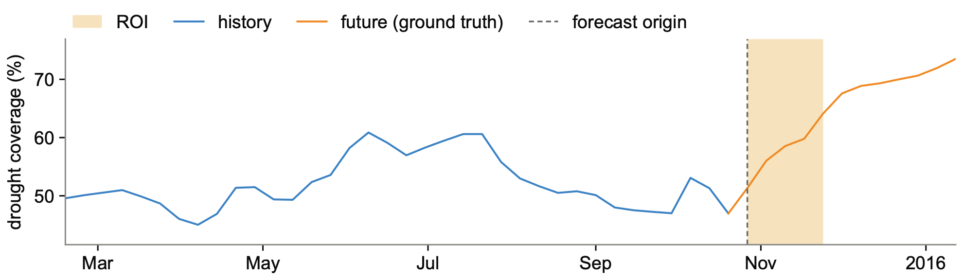
history future (ground truth) event window (ROI) — sample F03 of MMTR: hourly California freeway traffic around Thanksgiving Day 2016

Abstract

Time series from real-world systems are often accompanied by text, such as a report on an event that affects them. Two common tasks on these series are understanding, e.g., answering questions about a series, and forecasting its future values. Both tasks require reasoning over the series and the text together. Moreover, understanding outputs text while forecasting outputs a time series, so serving both requires a model that reads and generates both modalities. Large language models (LLMs) read time series as digit tokens and handle long series poorly. Time series foundation models (TSFMs) forecast well from large-scale pretraining but typically neither read nor generate text. Time series language models add a time series modality to the LLM but forecast on the LLM side, leaving the TSFM’s pretrained forecasting ability unused. We present TimeOmni-o1, which couples a pretrained TSFM and an LLM bidirectionally. In one direction, the TSFM encodes the series in compressed form for the LLM, which reasons over it together with the text. In the other, the LLM’s reasoning is fed back into the TSFM, which produces the forecast conditioned on it. One model architecture thus reads and generates both series and text, reasons in text, and draws on the TSFM’s pretrained forecasting ability. To train it, we build MMTR, a multimodal time series reasoning dataset with annotated reasoning traces, covering both tasks across 12 domains with 500k+ samples. On MMTR, TimeOmni-o1 outperforms existing models on both understanding and forecasting across most domains, as well as the LLM and the TSFM inside it when used individually. The gains carry over to three open benchmarks, where it outperforms the dedicated time series models.

Model

TimeOmni-o1 performs both the understanding and the forecasting task with one architecture (Figure 1). The input is a multivariate time series of $C$ channels, paired with a textual context: a question, background, or an event description. For understanding, the model generates a reasoning trace followed by a textual answer. For forecasting, the trace instead ends in a forecast instruction, and the output is a quantile forecast over the requested horizon, the window of future steps each sample specifies. The instruction states the window over which the event is expected to act, and the direction, shape and relative magnitude of its effect within that window.

Both task types share one workflow in which each component performs the function it was pretrained for: the LLM generates all text, and the TSFM encodes the time series and produces the forecast. The two components are coupled bidirectionally, with one pathway in each direction. On the series-to-LLM pathway, the TSFM maps the time series to patch representations, which are compressed into a bounded soft prompt that the LLM reads alongside the context to generate the trace and the answer or instruction. On the LLM-to-TSFM pathway, used for forecasting, the LLM’s hidden states are compressed and injected into the TSFM, which produces the forecast conditioned on them.

Overview of TimeOmni-o1: the TSFM and the LLM coupled in a loop, an understanding example and a forecasting example — Figure 1. Overview of TimeOmni-o1. Left: a pretrained TSFM and an LLM are coupled bidirectionally. The TSFM is the interface for time series, taking the input series and producing the forecast, and the LLM is the interface for text, taking the context and producing the reasoning trace and the answer. Middle: for understanding, the LLM reasons over the TSFM-encoded time series and the context text, and generates the reasoning trace and the answer. Right: for forecasting, the time series enters through the TSFM (1, 2) and the LLM generates the reasoning trace (3). The LLM’s hidden states over the whole sequence, holding the time series, the context, and the trace, are then fed back into the TSFM (4), which generates the quantile forecast (5).

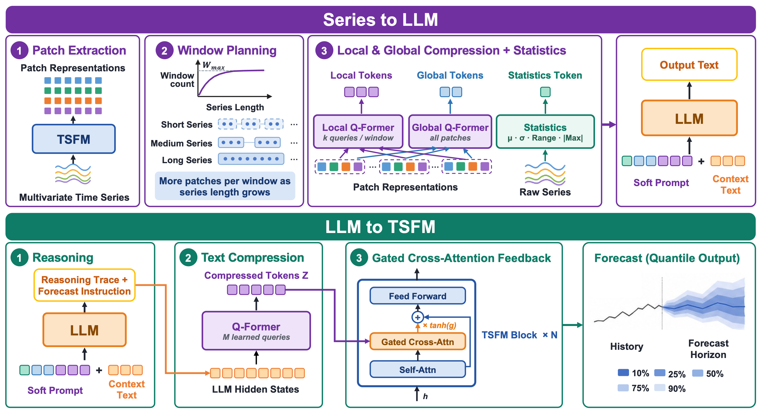
Series to LLM. To process long time series, the series-to-LLM pathway compresses the TSFM’s patch representations into a bounded soft prompt of local, global, and statistics tokens, which the LLM reads alongside the context (Figure 2, top). LLM to TSFM. The LLM-to-TSFM pathway compresses the LLM’s hidden states and injects them into every TSFM block through gated cross-attention, so the forecast is conditioned on the reasoning (Figure 2, bottom).

The two pathways of TimeOmni-o1: series to LLM on top, LLM to TSFM at the bottom — Figure 2. The two pathways of TimeOmni-o1. Top, time series to LLM: the TSFM maps the time series into patch representations (1). A planning rule sets the window count from the time series length (2). The Q-Former compresses the patches into local and global tokens; with the statistics token they form the soft prompt (3), which the LLM reads alongside the context text. Bottom, LLM to TSFM: the LLM generates the reasoning trace and the forecast instruction (1). The feedback Q-Former compresses the LLM hidden states into $M$ tokens $\mathbf{Z}$ (2). Gated cross-attention injects $\mathbf{Z}$ into every TSFM block (3), and the TSFM generates the quantile forecast.

Dataset: MMTR

Table 1 collects the related multimodal time series corpora, and no corpus in it combines a reasoning trace on every sample, both task types and real-world time series. We therefore build MMTR, a multimodal time series reasoning dataset with annotated reasoning traces, covering both the understanding and the forecasting task. It holds 573,653 samples: 568,586 for the understanding task over 12 domains and 5,067 for the event-conditioned forecasting task over 5 domains.

Table 1. MMTR against related multimodal time series corpora. The full comparison, including all eleven source corpora of MMTR, is the full comparison table in the paper’s appendix. Und. / Fc.: the corpus poses understanding / forecasting tasks. Trace: every sample carries an annotated reasoning trace; partial: only a subset does (2.3k of TSR-Suite’s 23.6k samples). Domains: as counted by the source. Series: real, synthetic, or both. Train split: the corpus has a training split, rather than being an evaluation-only benchmark. Samples: total instances as reported by the source.

Dataset	Und.	Fc.	Trace	Domains	Series	Train split	Samples
OpenTSLM CoT sets	✓	×	✓	1	real	✓	326k
RATs40K	✓	×	✓	10	real	✓	39.6k
ST-Bench	✓	✓	✓	10	synthetic	✓	28.2k
TSR-Suite	✓	✓	partial	10	real	✓	23.6k
TSQA	✓	✓	×	12	both	✓	193k
SciTS	✓	✓	×	12	both	✓	52.1k
Time-MMD	×	✓	×	9	real	✓	17.1k
CiK	×	✓	×	7	both	×	355
MMTR (Ours)	✓	✓	✓	12	both	✓	574k

Understanding task

The understanding task is built from six public reasoning-annotated corpora: the OpenTSLM chain-of-thought sets (Langer et al., 2026), ST-Bench (Ni et al., 2026), RATs40K (Yang et al., 2026), TSRBench (Zhou et al., 2026), TelecomTS (Feng et al., 2026) and HiTSR (Ding et al., 2026). They are unified into one schema of time series, question, reasoning trace and answer. The questions cover open question answering, multiple choice, classification, anomaly detection and diagnosis, and multi-step numerical calculation. The samples span 12 domains: physiology, telecommunications, urbanism, information technology, neuroscience, earth science, meteorology, economics, bioacoustics, manufacturing, energy, and synthetic data.

Forecasting task

The forecasting task is event-conditioned. Each sample pairs a time series history with a background and the description of an event (e.g., a heatwave alert, a holiday, a market event), and asks for a forecast over a horizon. The time series and their accompanying texts are collected from five public multimodal forecasting sources: CGTSF (Wang et al., 2025), Fidel-TS (Xu et al., 2025), MTBench (Chen et al., 2025), News Forecast (Wang et al., 2024) and Time-MMD (Liu et al., 2024). These sources contribute ten subsets in five domains: solar power, grid load, traffic flow, finance and climate. They carry no reasoning annotations, so we annotate every sample with Claude Sonnet 4.6 to add an event description condensed from the accompanying text, a reasoning trace, and a forecast instruction. The annotator writes the reasoning trace and the forecast instruction from the history and the event while seeing the future values, so the instruction matches the realized future, but it is prompted not to cite any specific future value. The window stated in the instruction, over which the event is expected to act, is the event region of interest (ROI). We record it as a separate field in each sample for ROI-weighted training and ROI evaluation. The subsets and the annotation protocol are detailed in Annotation and human review.

Table 2. Provenance of the forecasting task of MMTR. Time series are taken from ten subsets of five public multimodal forecasting sources; the background, event description, reasoning trace, forecast instruction and ROI are annotated in this work. History and Horizon: window lengths in steps; the equities windows vary with the trading session and are reported as medians. Sources as cited in the Forecasting Task section.

Source	Subset	Domain	Resolution	History	Horizon
CGTSF	MSPG, Melbourne PV	Solar	15 min	480	96
CGTSF	PTF, Paris traffic	Traffic	hourly	120	24
Fidel-TS	50Hertz renewable	Solar	15 min	288	96
Fidel-TS	Calgary PV	Solar	hourly	96	24
Fidel-TS	California ISO	Load	5 min	576	288
MTBench	US equities	Finance	intraday	390	78
News Forecast	Australian load	Load	30 min	48	48
News Forecast	California traffic	Traffic	hourly	120	48
News Forecast	Bitcoin	Finance	daily	60	14
Time-MMD	US drought	Climate	weekly	36	12

Annotation and human review

Annotation protocol. The 5,067 collected samples (4,630 training and 437 test) are annotated by an LLM annotator, Claude Sonnet 4.6. Annotation runs in two stages, separated by what each field is used for. The event description is a model input at test time, so the first stage must not depend on the future. In this stage the annotator receives a hand-written dataset background, the sample’s accompanying text and the timestamps of the history and the horizon; it receives neither the time series nor any future value. The accompanying text is the source’s own aligned text rather than retrieved material: weather forecasts and reports for the solar and load sets, aligned news for the finance and traffic sets, and drought reports for the climate set. Text dated inside the forecast horizon is marked, and the annotator is instructed to ignore it. The annotator returns the event description, condensed from the accompanying text without causal phrasing. The reasoning trace, the forecast instruction and the ROI are training targets and are written by the annotator in the second stage. The instruction names the ROI and states the direction, shape and relative magnitude of the effect in words. Here the annotator receives the background, the event description of the first stage as a fixed input, the window metadata, a rendering of the time series, and the future window as a timestamped value table. Three constraints are imposed on the second stage: the ROI lies inside the horizon, the trace uses the history and the event only, and no future value is cited. A schema check enforces the ROI bounds, and an automatic check flags any quoted future value.

Trace quality is checked by human review. Two independent reviewers rate 1,000 traces, sampled with stratification by task and domain, against the input time series, the context, and the annotated answer. A trace fails if its reasoning contradicts the time series, the context, or the final answer, or if it contains a factual error. On average, 93.3% of the understanding traces and 97.7% of the forecasting traces pass, and the two reviewers give the same pass/fail label for 96.6% of the traces. The review protocol and the per-task pass rates are given in the paper’s appendix.

Samples from MMTR

This section shows one sample per domain of the understanding task (U01 to U12) and one per domain of the forecasting task (F01 to F05). Questions and traces are abridged: option lists, category inventories and formatting instructions are shortened, and the values cited by the traces are checked against the stored series. Each understanding card shows the time series, the question, the annotated reasoning trace and the answer. Each forecasting card shows the history and the future ground truth with the ROI shaded, then the dataset background, the event description, the reasoning trace and the forecast instruction. Markers in the figures mark the values the trace cites.

U01 Physiology U02 Telecommunications U03 Synthetic U04 Urbanism U05 Information technology U06 Neuroscience U07 Earth science U08 Meteorology U09 Economics U10 Bioacoustics U11 Manufacturing U12 Energy F01 Solar F02 Load F03 Traffic F04 Finance F05 Climate

Understanding task

U01

Physiology

OpenTSLM ECG-QA

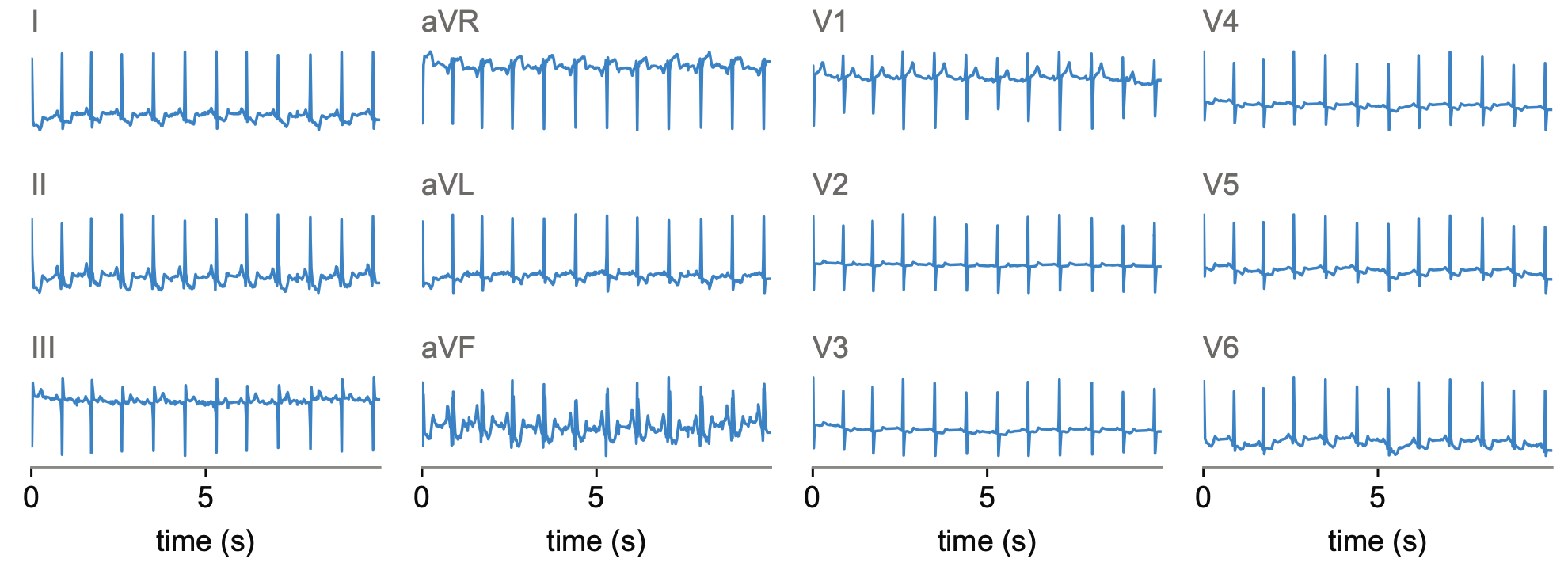
Open-ended diagnostic question answering; 12-lead ECG, 10 s at 500 Hz (5,000 points per lead).

Question: Clinical context: 72-year-old female; 12-lead clinical ECG (baseline drift, static/burst noise and electrode artefacts noted; extra beats; pacemaker present). Which diagnostic symptom does this ECG show: myocardial infarction in inferoposterolateral leads, or myocardial infarction in anteroseptal leads (including uncertain symptoms)?
Reasoning trace: Baseline drift and noise may obscure details and the pacemaker can affect some features, but the focus is on infarction patterns. The notable changes appear in the inferoposterolateral leads (II, III, aVF and possibly V5-V6), which show ST-segment elevation or other ischaemic changes; an anteroseptal infarction would instead involve V1-V4. Together with the clinical context this supports an inferoposterolateral myocardial infarction.
Answer: myocardial infarction in inferoposterolateral leads

U02

Telecommunications

TelecomTS

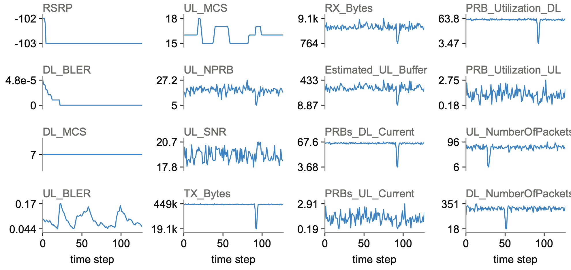
Network-level activity recognition; 16 KPI channels over 128 steps.

Question: A 5G monitoring window with 16 KPI channels. Observation summary (abridged): RSRP stable but weak ($-$103 to $-$102 dB); uplink SNR 17.8-20.7 dB; UL_MCS 15-18 while DL_MCS is constant at 7; DL_BLER negligible, UL_BLER 0.044-0.17; downlink PRBs about 63 with a sharp drop to single digits late in the trace, uplink PRB use minimal; traffic uplink-dominant and bursty (TX_Bytes 19 k-449 k with a sharp dip, RX_Bytes 0.8 k-9 k); the estimated uplink buffer is often large (mean 296 KB); 100% TCP in both directions. Which type of activity occurred: YouTube viewing, Twitch stream, or file transfer?
Reasoning trace: The radio link is stable but weak (RSRP about $-$103 dB) with a consistent uplink SNR (about 19.2 dB); uplink MCS varies slightly while downlink MCS stays constant. Traffic is highly uplink-bursty, with TX_Bytes dropping sharply, and the estimated uplink buffer stays high, indicating queued data. This pattern is consistent with a file transfer.
Answer: File download was the activity.

U03

Synthetic

HiTSR, level 3

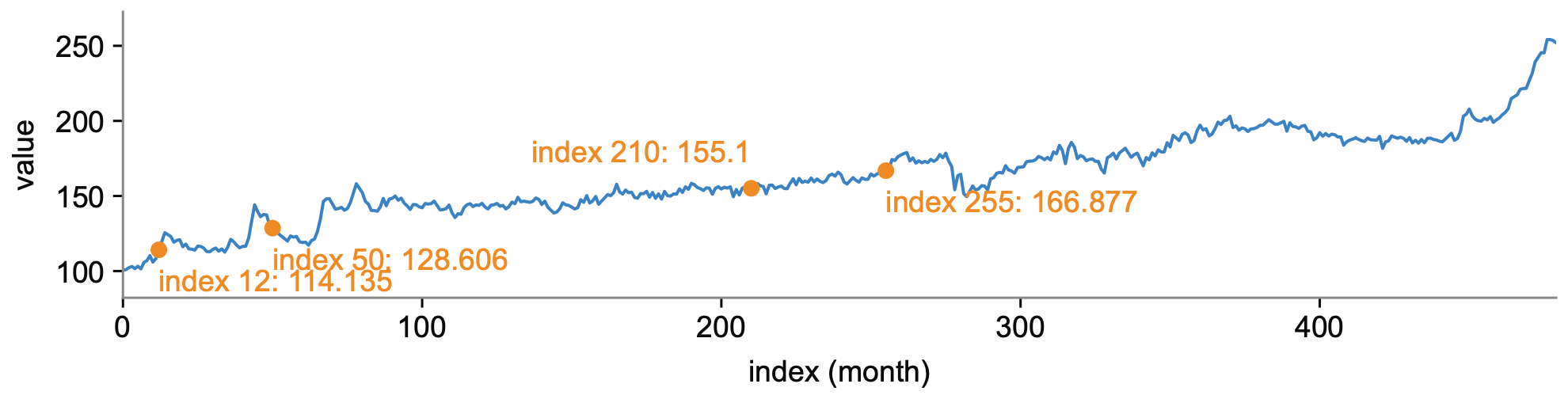
Multiple choice matching pattern, values and semantics; univariate, 480 monthly points.

Question: Which statement best describes the long-term behaviour of this monthly retail broiler composite series and confirms a specific value? A. A clear upward trend with no seasonal component; the value at index 255 is 166.877. B. Strong periodic seasonality with a 12-month cycle; the value at index 12 is 114.135. C. A monotonic decrease after index 200; the value at index 210 is 155.1. D. Roughly constant around 150 for the first 100 months; the value at index 50 is 128.606.
Reasoning trace: A: the series rises over the long run, most steeply beyond index 250, with no consistent seasonal pattern; index 255 is exactly 166.877; a gradual price increase in the broiler market is plausible. B: peaks and troughs do not recur annually, so the 12-month seasonality claim fails even though 114.135 at index 12 is correct. C: values climb above 250 late in the series, contradicting a monotonic decline, although 155.1 at index 210 is correct. D: the series starts near 100 and drifts up to about 140 by index 100, so it is not constant around 150; 128.606 at index 50 is correct.
Answer: A

U04

Urbanism

ST-Bench

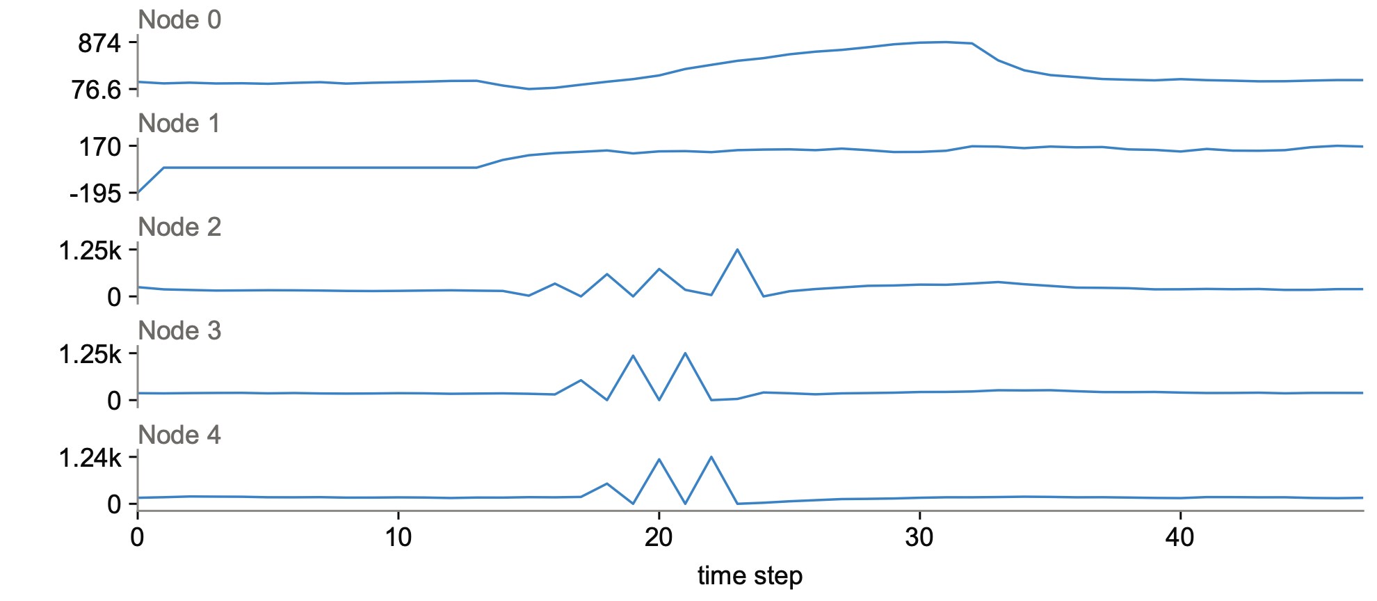
Spatio-temporal graph reasoning, entity identification; 5 graph nodes over 48 steps with edges 0$\to$2, 1$\to$2, 2$\to$3, 3$\to$4, 4$\to$2.

Question: Five nodes each carry a length-48 series; graph edges: Node 0$\to$2, 1$\to$2, 2$\to$3, 3$\to$4, 4$\to$2. Which (name, description) pair should Node 3 correspond to? A. Central Square, main city square intersection; B. Highway Exit, major highway exit point; C. Ring Road, ring road junction; D. Bypass Junction, peripheral traffic bypass point.
Reasoning trace: Graph: Node 2 is a convergence point fed by Nodes 0 and 1, then flows to Node 3 $\to$ Node 4 $\to$ back to Node 2 (a loop). Series: Node 0 surges from about 76 to about 874 around indices 15-33; Node 1 is zero for indices 1-13 and then holds 60-170; Node 2 is erratic with extreme spikes (1250, 731, 593); Node 3 has a stable 150-200 baseline, extreme spikes (1184, 1250) near indices 17-23, then stabilises higher (180-265); Node 4 mirrors Node 3 with spikes (1242, 1178) followed by very low values (28, 66, 96). Node 3 receives the converged flow, carries the major surge, and sits on the circular 2$\to$3$\to$4$\to$2 structure, so it is a junction on a ring road rather than the central convergence point itself.
Answer: C (Ring Road, ring road junction)

U05

Information technology

TSRBench

Rule-based anomaly detection; univariate, 256 points (Kubernetes cluster autoscaler metric).

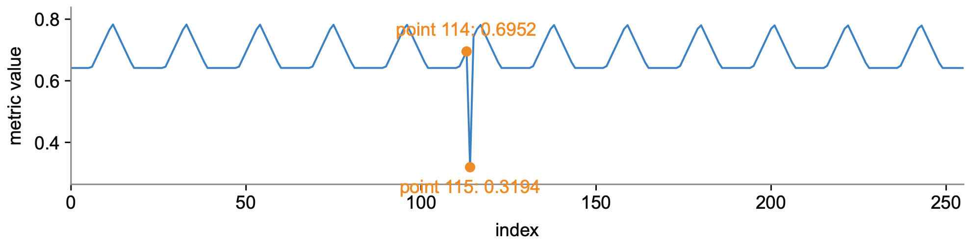
Question: Cluster Autoscaler Metrics collected from a Kubernetes cluster, length 256. Given that a sudden drop of more than 0.3 is considered anomalous, should the series be considered anomalous near point 114?
Reasoning trace: Step 1: this is anomaly detection with an explicit rule (a drop larger than 0.3). Step 2: the relevant patterns are the drop magnitude, the 0.3 threshold and the location near point 114. Step 3: the value at index 114 is 0.6952 and the next value (index 115) is 0.3194, a drop of 0.3758 that exceeds the threshold; the drop is abrupt relative to the cyclical pattern (peaks about 0.78, troughs about 0.64). Steps 4-5: the gradual cyclical rises and falls do not explain such an abrupt drop, so the rule is unambiguously violated. Step 6: a drop of 0.3758 directly adjacent to point 114 qualifies as an anomaly.
Answer: Yes

U06

Neuroscience

OpenTSLM Sleep

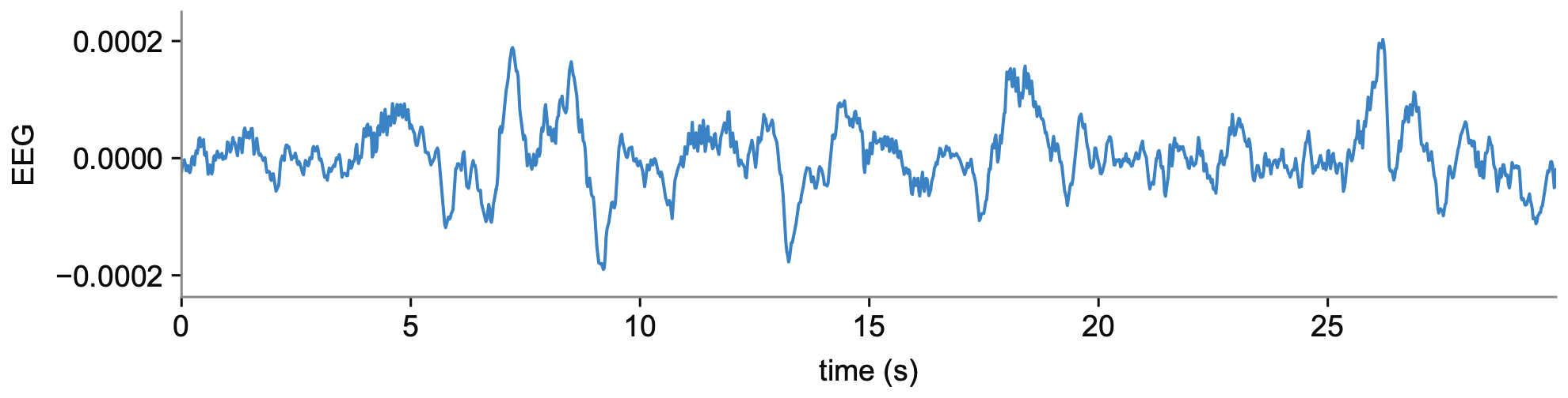
Sleep-stage classification; single-channel EEG, one 30-s epoch (1,500 points).

Question: A 30-second EEG segment corresponds to one of two sleep stages: Non-REM stage 4 or Wake. Determine the stage from the signal alone, reasoning in a single paragraph and ending with the answer.
Reasoning trace: The signal shows relatively slow oscillations with large amplitude variations, indicating synchronised neuronal activity. Such slow-wave activity is the hallmark of deep sleep; a wakeful state would instead show faster, lower-amplitude, desynchronised activity. The segment therefore matches a deep sleep stage rather than wakefulness.
Answer: Non-REM stage 4

U07

Earth science

RATs40K

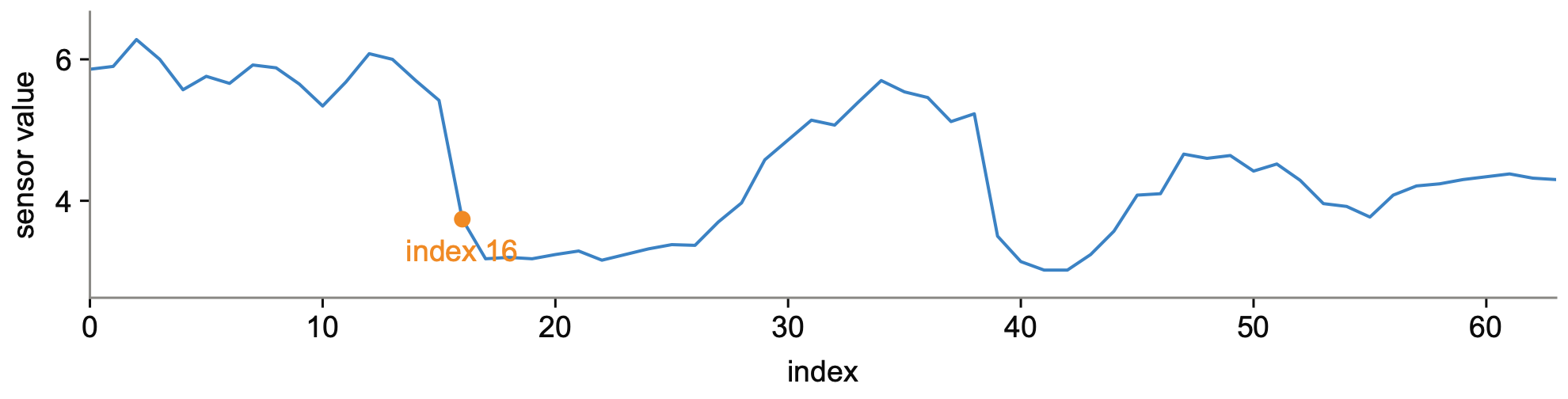
21-way anomaly diagnosis; univariate, 64 points (environmental sensor).

Question: A univariate series of length 64 collected from an environmental sensor. Analyse the temporal dynamics and name the category that best describes it, choosing from: Amplitude, Change Point, Collinearity Shift, Continuous Segment, Covariance Structure, Distributional Change, Drift, Joint Space, Nonlinear Pattern, Pattern Change, Periodic Change, Point, Principal Component Space, Repeated Value, Sparse, Sudden Flatline, Sudden Spike, Temporal Dependency, Trend Change, Trend Divergence Anomaly, or Normal Sequence.
Reasoning trace: The series initially fluctuates within a stable range (about 5.5-6.3). Starting at index 16 the values drop to a lower range (about 3.0-3.4), an abrupt shift in both mean and variance that marks a change point. There is some later recovery and fluctuation, but the initial drop is a clear change in statistical behaviour.
Answer: Change Point Anomaly

U08

Meteorology

RATs40K

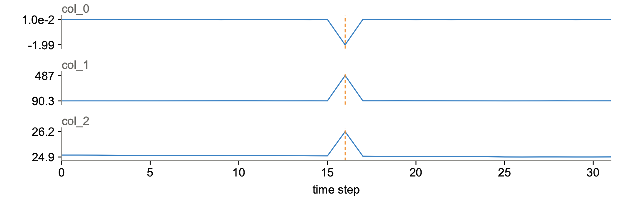
Multivariate anomaly diagnosis, 7-way; 3 variables over 32 steps (Tropical Atmosphere Ocean buoy array).

Question: A multivariate series with 3 variables (col_0, col_1, col_2), each of length 32, collected from ocean / tropical-atmosphere buoy observations. Which category best describes it: Collinearity Shift, Covariance Structure, Joint Space, Principal Component Space, Temporal Dependency, or Trend Divergence Anomaly, or Normal Sequence?
Reasoning trace: col_0 stays near zero with small fluctuations but drops abruptly to $-$1.99 at time step 16. col_1 progresses smoothly but spikes to 487.0 at the same step. col_2 trends gradually downward but jumps to 26.2 at step 16. Each variable is individually anomalous at step 16, and their joint configuration there is inconsistent with the expected multivariate relationships, indicating a system-level disturbance.
Answer: Joint Space Anomaly

U09

Economics

TSRBench

Multi-step numerical calculation, counting events; univariate, 256 daily points.

Question: Daily Customer Engagement (Marketing & Sales), 256 points starting 1 October 2024. The company ran a series of marketing campaigns; during the period engagement showed a series of rapid spikes each followed by a quick decline. How many such spike-and-decline events occurred, and what could have caused them?
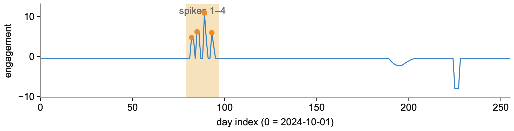
Reasoning trace: Step 1: count distinct ‘rapid spike followed by quick decline’ events. Step 2: a spike must clearly exceed the baseline (about $-$0.47), consecutive spike days form one event, and the decline must return to baseline within 1-2 days. Step 3: spike 1 on days 82-83 (4.71, 4.71, then $-$0.48); spike 2 on days 85-86 (6.13, 6.14, then $-$0.47); spike 3 on days 89-90 (10.82, 4.30, then $-$0.48); spike 4 on days 93-94 (5.90, 2.71, then $-$0.47). Step 4: four events. Step 5: no overlapping events; the later negative excursions (e.g. $-$8.05) are downward anomalies, not engagement spikes. Step 6: four spike-decline events, consistent with campaign launches.
Answer: 4

U10

Bioacoustics

TSRBench

Binary classification, call present or absent; 2-s hydrophone waveform.

Question: An audio segment may contain a North Atlantic right whale up-call (about 60-250 Hz, lasting about 1 s); the low-frequency band is often congested with ship noise, drilling or piling. The 2-second waveform is sampled at 2 kHz. Does the segment contain a right whale call? (a) Right Whale Present, (b) No Right Whale.
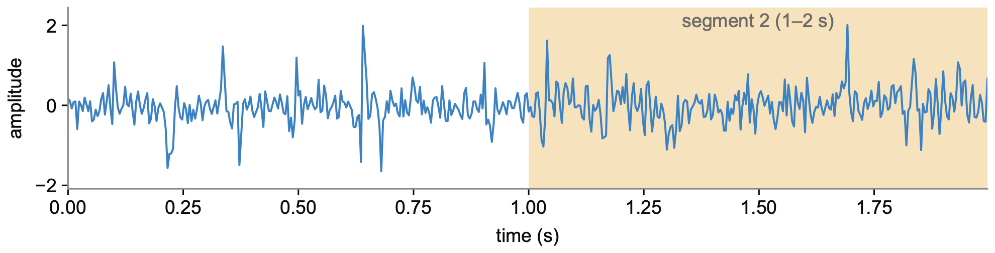
Reasoning trace: Step 1 (task intent): binary classification of whether a 2-s segment contains an up-call defined by its 60-250 Hz band and about 1 s duration. Step 2 (key patterns): frequency range, duration, amplitude consistency (a gradually rising ‘up-call’ envelope rather than impulsive noise), and anthropogenic interference. Step 3 (analysis): split the waveform into two 1-s segments. Segment 1 (0-1 s) has scattered in-band energy and strong energy below 60 Hz, typical of ship noise. Segment 2 (1-2 s) shows a sustained energy concentration at 90-180 Hz for about 1 s, matching the band and duration of an up-call. Step 4: segment 2 satisfies the band and duration criteria. Step 5 (reflection): the largest excursions of segment 1 (near 0.2 s and 0.7 s) are short and broadband, not a sustained tone; segment 1 lacks spectral focus. Step 6: the sustained, band-limited, about-1-s component in the second half identifies an up-call.
Answer: Right Whale Present

U11

Manufacturing

RATs40K

21-way anomaly diagnosis; univariate, 64 points (machine system).

Question: A univariate series of length 64 collected from a machine system. Analyse the temporal dynamics and name the category that best describes it (same 21 categories as above).
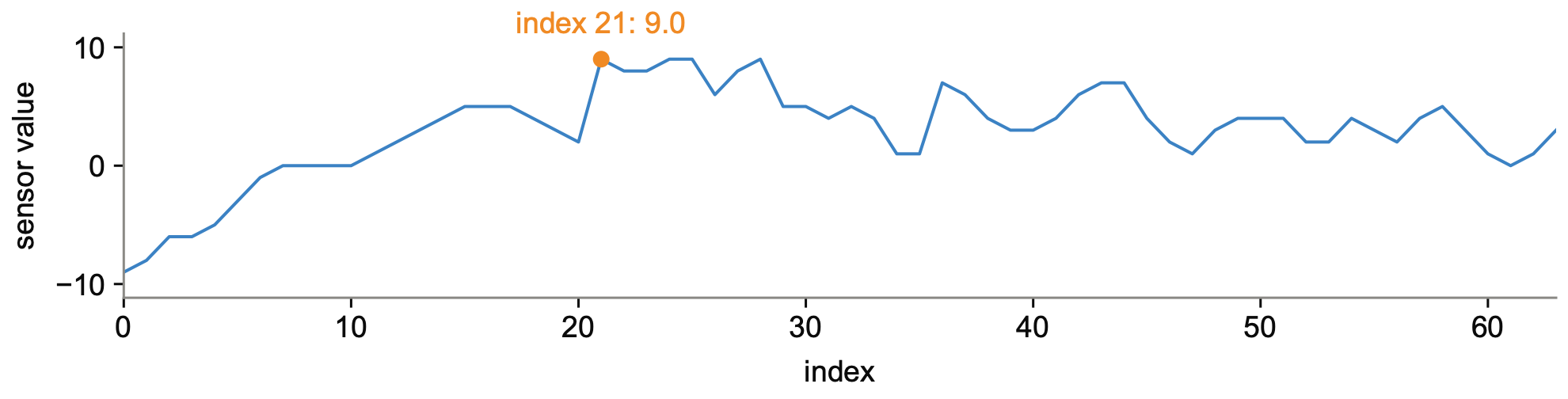
Reasoning trace: Several irregularities are present: a flatline of zeros at indices 7-10, repeated values (5.0 at indices 15-17, 8.0 at indices 22-23), and fluctuating segments without a consistent trend. The most prominent, however, is the sudden jump to 9.0 at index 21.
Answer: Sudden Spike Anomaly

U12

Energy

TSRBench

Appliance-signature classification; univariate, 720 points (2-min sampling over 24 h).

Question: Electricity usage of a UK household from the ‘Powering the Nation’ study, sampled every 2 minutes over 24 hours (720 points). Classify the device usage pattern: (a) Desktop or (b) Laptop.
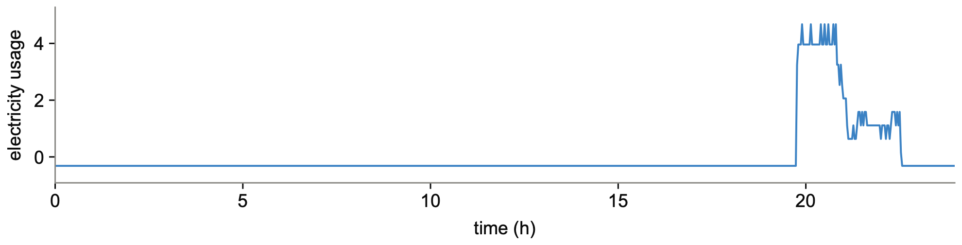
Reasoning trace: Step 1: binary classification of a device energy signature. Step 2: key patterns are the baseline level, the duration of sustained high consumption, and volatility. Step 3: the signal sits at one repeated low value ($-$0.3151) for 636 of the 720 points; the only active block runs from index 593 to 676 (about 168 minutes), holds 3.96 to 4.67 for about 62 minutes, then steps down through 3.25, 2.06, 1.11 and 0.64; transitions such as 1.59 $\to$ $-$0.32 are abrupt. Step 4: an idle baseline for most of the day, a single active block of under three hours and stepped power levels match a laptop (battery-driven power management) rather than a desktop’s steady higher load over a working day. Step 5: the 4.67 readings are single 2-minute points inside the block, not a sustained higher load. Step 6: Laptop.
Answer: Laptop

Forecasting task

F01

Solar

CGTSF, MSPG Melbourne PV

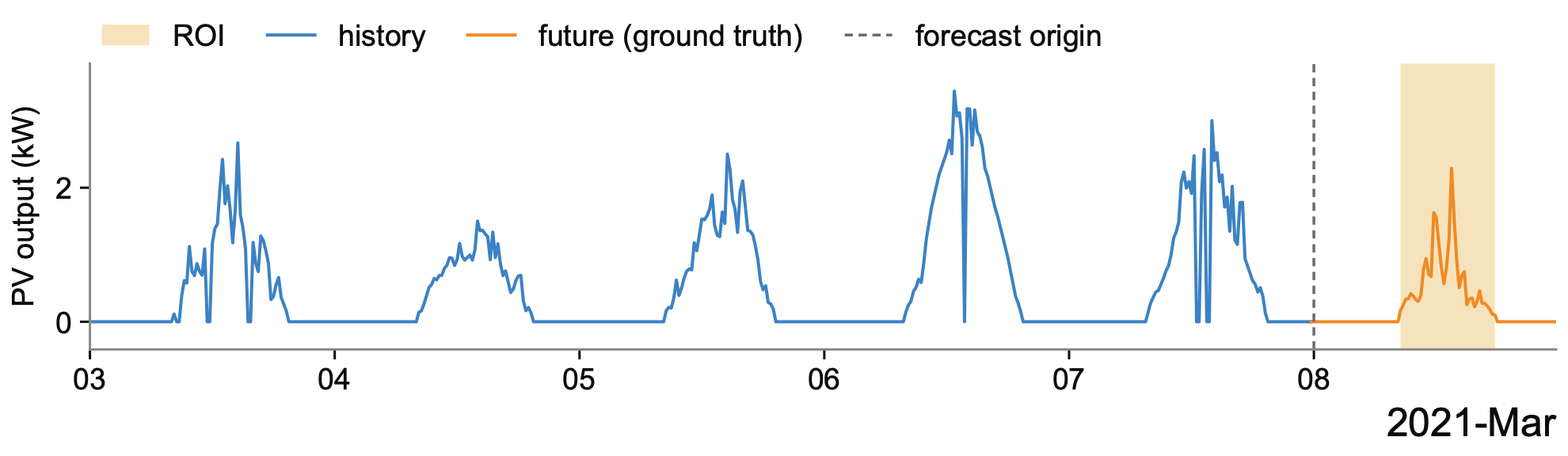
Event-conditioned forecasting; 15-min resolution, history 480 and horizon 96 points; ROI [514, 552), 08:30 to 17:45 on 8 March 2021.

Background: Power generated by a single photovoltaic site in Melbourne, Australia, every 15 minutes. Output follows a daily bell shape (zero overnight, peak near solar noon) whose height and smoothness are gated by cloud, rain and haze.
Event: Monday, 8 March 2021 is the target day. Conditions: moderate drizzle with a gentle breeze, 14-19 C; sunrise 06:11, sunset 18:50.
Reasoning trace: The span from 08:30 (row 514) through 17:45 (row 551) covers the generation window of the target day, inside the sunrise-to-sunset interval given by the event. Moderate drizzle through the whole day places it among the low days of the history window, whose output stays well below the highest day. Those low days do not form a smooth bell: output is uneven all day, with isolated readings well above their neighbours. The target day follows the same profile, low and erratic with at most brief isolated higher readings, and falls to zero before sunset.
Forecast instruction: Over index range [514, 552), solar generation remains at a persistently low, erratic level throughout the active generation window, with a brief pronounced peak in the early afternoon forming the single highest reading of the day, before declining back to low irregular values and reaching zero before sunset. Overall, with drizzle reported, the peak stays well below the series’ typical highs.

F02

Load

Fidel-TS, California ISO

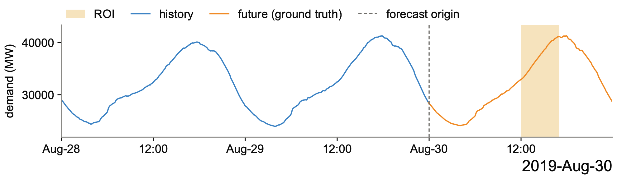
Event-conditioned forecasting; 5-min resolution, history 576 and horizon 288 points; ROI [720, 781), 12:00 to 17:00 on 30 August 2019.

Background: California ISO grid electricity demand in megawatts, every 5 minutes. The dominant pattern is a daily cycle (overnight trough, daytime rise, evening peak) shaped by temperature-driven heating and cooling load.
Event: Forecast for California on 30 August 2019: warm and sunny, 18-23 C, partly sunny with a gentle west breeze; temperatures rise through the day to an afternoon high, then ease slightly in the evening under clear skies.
Reasoning trace: The selected span runs from 12:00 to 17:00 on 30 August, matching the afternoon period when temperatures keep rising to their daily high. In the history window demand follows a recurring daytime build toward a late-day high. With warm, sunny conditions persisting into the afternoon, the future window keeps climbing through this interval and finishes at its highest point before the evening easing begins.
Forecast instruction: [720, 781) shows a sustained afternoon climb that ends close to the daily peak, after which demand levels off and turns down. Overall, under sunny skies, output reaches roughly its usual peak level.

F03

Traffic

News Forecast, California traffic

Event-conditioned forecasting; Hourly resolution, history 120 and horizon 48 points; ROI [120, 143), 00:00 to 22:00 on 24 November 2016.

Background: Hourly traffic volume on a California freeway segment. The dominant patterns are a daily commute cycle (morning and evening peaks) and a weekly cycle (weekdays heavier than weekends); public holidays reshape the weekday pattern.
Event: Thanksgiving Day, a US public holiday, falls on 24 November 2016 within the future window. The accompanying regional news headlines (16-17 November) contain no road-specific event.
Reasoning trace: The relevant span is 24 November 00:00 through 22:00, Thanksgiving Day inside the future window. In the history window this freeway follows a stronger weekday commute cycle, but the holiday note points to a weekend-like profile instead: a muted build through the morning, a broad high around midday, and an easing later in the day rather than a pronounced commuter pattern.
Forecast instruction: [120, 143) shows a gradual daytime rise to a midday crest followed by an uneven decline through the evening. Overall, on the holiday, the midday crest stays far below the usual weekday peaks.

F04

Finance

MTBench, US equities

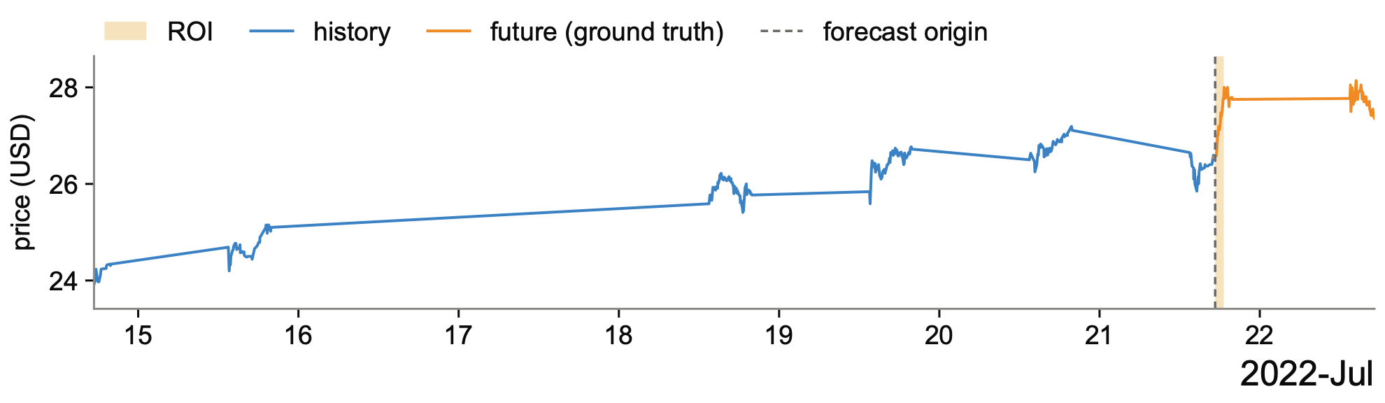
Event-conditioned forecasting; Intraday resolution, history 389 and horizon 78 points; ROI [389, 406), 17:19 to 18:36 UTC on 21 July 2022.

Background: Intraday price of a single US-listed stock over about one trading week of higher-frequency points, in US dollars. Moves are driven by company news, earnings and broad market sentiment, with no within-window seasonality.
Event: On 21 July 2022 at 17:15 UTC, Dorchester Minerals, L.P. (Dallas, Texas) announced its second-quarter 2022 cash distribution, covering the three months ended 30 June 2022 and payable on 11 August 2022 to unitholders of record as of 1 August 2022.
Reasoning trace: The selected span runs from 17:19 to 18:36 on 21 July, the first 75 minutes after the 17:15 announcement, so it holds the initial reaction to the cash distribution. A cash distribution is positive news for unitholders, and the last hours of the history window are flat, so the reaction is an advance from a calm base. That base sits near the top of the week’s range in the history window, so an advance carries the series close to or above its previous highs.
Forecast instruction: In [389, 406), the future window shows a sustained upward run that ends at its highest point and levels off afterward. Overall, the run ends slightly above the series’ previous highs.

F05

Climate

Time-MMD, US drought

Event-conditioned forecasting; Weekly resolution, history 36 and horizon 12 points; ROI [36, 41), 27 October to 24 November 2015.

Background: Share of US land area under drought (US Drought Monitor categories D0-D4), in percent, reported weekly. It moves slowly and persistently: coverage builds over dry spells and recedes after sustained rain or snow, lagging precipitation by weeks.
Event: Monthly precipitation reports for April-September 2015 (all before the horizon): April was the 37th wettest on record, May the wettest month ever recorded for the contiguous US (4.36 in), June the 9th wettest and July the 14th wettest (about 26% of the US in moderate-to-exceptional drought as of 31 July). August turned dry (28th driest, 0.26 in below average) and the national drought footprint expanded; September was the 21st driest (0.40 in below average).
Reasoning trace: The ROI spans 27 October (row 36) through 24 November 2015 (row 40), the first month of the future window. Both August and September were below average in precipitation and the drought footprint was already expanding at the close of August; coverage lags precipitation by weeks, so this deficit is due to appear in the weeks after the horizon. The history window does not show it yet: coverage fell from its July high to a local low at the horizon. Two consecutive dry months with the footprint already expanding point to a rise from that low sustained through the whole span, not a one-week uptick.
Forecast instruction: The ROI [36, 41) captures a rapid expansion of drought coverage from late October through late November 2015, ending at its highest point in that span. Overall, after two dry months, coverage ends above the highest level of the history window.

Case studies

This section presents two understanding cases and two forecasting cases; the statistics over the full test sets are those of Section 6.3 of the paper. Baselines are scored leniently throughout: an output counts as correct if the ground-truth phrase appears anywhere in it, a bare option letter counts, and the last number of a numeric answer is taken. In every quoted trace, the cited values are approximate, because the LLM reads the time series through the soft prompt rather than as digits; what is checked against the raw time series is the structural judgment: how many events, how large, and which shape.

Understanding cases

U1 Counting drops (TSRBench, Earth science)

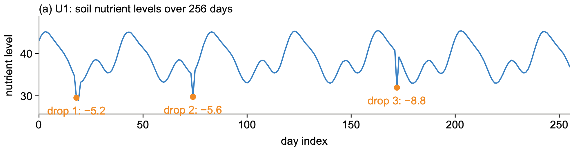
Case U1 — The three largest one-day drops, which the trace counts.

The question asks how many significant downward spikes in a 256-day soil-nutrient time series could critically impact plant growth; the answer is 3. The trace of TimeOmni-o1 sets a criterion first and then enumerates: it lists three drops of about 7 to 8 units with their days, and it names smaller declines that it rules out. Against the raw time series, exactly three one-day drops exceed 5 units (5.2, 5.6 and 8.8) and the fourth largest is 1.3. Every other model that produces a number is off by one (Table 3): the no-reasoning model and TimeOmni-1 answer 2, the fine-tuned LLM and TimeOmni answer 1, and Time-MQA detects only the first drop. The models that state a count directly undercount, whereas the trace counts the drops one by one against a stated criterion.

Question as posed

You are a time series analysis expert. This is a metric called Soil Nutrient Levels collected from Agriculture with length of 256:. In the context of Soil Nutrient Levels, considering the time series starts from the beginning of a growing season and each point represents a day, how many significant downward spikes in nutrient levels occurred that could critically impact plant growth?

Reasoning trace generated by TimeOmni-o1

Step 1 Analyzing task intent:  
[Judgment] Significant downward spikes  
[Description] The problem requires counting "significant downward spikes" in soil nutrient levels that could "critically impact plant growth." Keywords like "significant," "downward spikes," and "critically impact" indicate the need to identify abrupt, severe drops in nutrient levels rather than gradual trends or minor fluctuations.  

Step 2 Selecting task-relevant key patterns:  
[Judgment] Amplitude deviation; Rate of change; Threshold deviation  
[Description]  
- **Amplitude deviation**: Measures the magnitude of a drop relative to preceding values. Critical for identifying "significant" spikes.  
- **Rate of change**: Detects abrupt declines (spikes) versus gradual decreases.  
- **Threshold deviation**: Uses domain knowledge (e.g., nutrient levels dropping below agronomic safety thresholds) to define "critical" impact.  

Step 3 Analyzing time series samples using selected key patterns:  
[Analysis]  
1. **Day 18–19**: Nutrient levels drop from **35.01** to **27.34** (Δ = **-7.67**). This is the largest single-day decline in the series, far exceeding typical fluctuations (usually ±1–3).  
2. **Day 64–65**: Drop from **33.72** to **26.98** (Δ = **-6.74**). Second-largest decline, comparable to agronomic critical thresholds.  
3. **Day 129–130**: Drop from **33.78** to **25.59** (Δ = **-8.19**). New maximum deviation, indicating a severe spike.  
Other fluctuations (e.g., Day 1–2, Day 90–91) show smaller declines (Δ < 5) or gradual trends, deemed non-critical.  

Step 4 Generating preliminary answers by combining task intent and key patterns:  
[Judgment] 3  
[Description] Three spikes (Days 18–19, 64–65, 129–130) exhibit abrupt declines (Δ > 6.7) exceeding typical variability and aligning with agronomic thresholds where nutrient levels fall below critical ranges for plant growth.  

Step 5 Enhancing answers through reflection:  
[Analysis]  
- Verified no other spikes met amplitude (>6.7) and rate-of-change criteria.  
- Confirmed domain relevance: Drops of ~7+ units in soil nutrients (e.g., nitrogen) are known to stress crops.  
- Ruled out gradual declines (e.g., Day 90–91: 32.97 → 32.83) as non-spikes.  

Step 6 Summarizing the thinking process to output the answer:  
[Description] The analysis identified three instances where soil nutrient levels dropped abruptly by >6.7 units, exceeding natural variability and agronomic critical thresholds. These spikes (Days 18–19, 64–65, 129–130) align with the definition of "significant downward spikes" capable of critically impacting plant growth.  
[Judgment] 3

Final answer 3

Raw outputs of the compared models

None (no reasoning)

Answer: 2

TimeOmni-o1's LLM (zero-shot)

Thinking Process:

1.  **Analyze the Request:**
    *   **Input:** A raw time series of 256 points (though truncated in the prompt, I need to work with the provided data).
    *   **Context:** Soil Nutrient Levels in Agriculture.
    *   **Timeframe:** Starts from the beginning of a growing season, each point is a day.
    *   **Task:** Identify the number of *significant downward spikes* in nutrient levels that could *critically impact plant growth*.
    *   **Role:** Time series analysis expert.

2.  **Analyze the Data:**
    *   The data provided is a single channel of 256 points (though the prompt says "1 channel, 256 points per channel" and then lists numbers, followed by "... (truncate […]

TimeOmni-o1's LLM (fine-tuned)

Step 1 Analyzing task intent:  
[Judgment] Significant downward spikes.  
[Description] The problem requires identifying "significant downward spikes" in soil nutrient levels that "critically impact plant growth." Keywords like "downward spikes" and "critically impact" indicate the focus is on abrupt, severe drops in nutrient levels, not gradual declines or minor fluctuations.  

Step 2 Selecting task-relevant key patterns:  
[Judgment] Amplitude of drop; rate of decline; deviation from local trend.  
[Description]  
- **Amplitude of drop**: A spike must involve a large absolute decrease in nutrient levels (e.g., >10 units) to qualify as "significant."  
- **Rate of decline**: A single-day d […]

TimeOmni (fine-tuned)

Answer: 1

TimeOmni-1-4B

Time-MQA-7B

Based on the data provided, there is one significant downward spike starting from day 18 where the value drops to 29.01, which is a considerable decrease from previous points that were around or above 40. This drop alone greatly impacts the consistency needed for soil nutrients. Subsequently, it could negatively impact plant growth significantly thereafter. Thus, the drop to 29.01 represents a substantial change that might harm plants.

TimeOmni-VL-15B

To answer this, I would look for sharp, isolated dips (downward spikes) in the series that last for a few data points and then return to a higher level. These would be the most significant as they represent rapid, critical declines in soil nutrients that could stifle plant growth.

Chat-TS-8B

[TS_TOKENS x33] The long-range forecast suggests:  SHAPE OUTPUT:(240, 24).

OpenTSLM-3B

(a)

ChatTime-1-7B

###0.0085### ###-0.0681### ###-0.1285### ###-0.1917### ###-0.2311### ###-0.2461### ###-0.2357### ###-0.1937### ###-0.1299### ###-0.0681### ###-0.0045### ###0.0377### ###0.0705### ###0.0743### ###0.0505### ###0.0053### ###-0.0475### ###-0.0817### ###-0.1013### ###-0.0977### ###-0.0587### ###-0.0011### ###0.0829### ###0.1735### ###0.2663### ###0.3627### ###0.4407### ###0.4795### ###0.4931### ###0.4863### ###0.4583### ###0.4347### ###0.3891### ###0.3535### ###0.3199### ###0.2753### ###0.2357### ###0.1889### ###0.1409### ###0.0851### ###0.0223### ###-0.0425### ###-0.1033### ###-0.1599### ###-0.2061### ###-0.2313### ###-0.2313### ###-0.2081### ###-0.1549### ###-0.0913### ###-0.0329### ###0.0223## […]

U2 Fine-grained diagnosis (RATs40K, Earth science)

Case U2 — A gradual decline with one partial rebound and no jump, spike or change of variance.

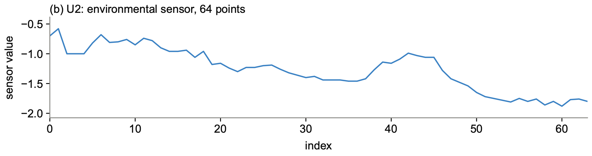
The 21-way question asks which category describes a 64-point environmental-sensor time series; the answer is normal sequence. The time series declines from $-0.70$ to $-1.80$ with one partial rebound around index 40 and no jump, spike or change of variance; in the source taxonomy a drift anomaly requires a systematic departure from a baseline, not a gradual decline. Every other model that produces a category reports drift (the no-reasoning model, the fine-tuned LLM, TimeOmni, TimeOmni-1 and Time-MQA), and TimeOmni-VL reports trend divergence. The trace of TimeOmni-o1 checks for disruptions, spikes and irregularities first and assigns the category only then. The same pattern holds over the 453 univariate RATs40K test samples: 188 are normal, the no-reasoning model labels 132 of them normal and predicts drift 96 times against 58 true, and TimeOmni-o1 labels 177 normal and predicts drift 62 times.

Question as posed

You are a time series anomaly diagnosis expert. The following is a univariate time series of length 64, collected from Environment-Sensor.

Analyze the temporal patterns and determine which of the following categories best describes this sequence:
- Amplitude Anomaly
- Change Point Anomaly
- Collinearity Shift Anomaly
- Continuous Segment Anomaly
- Covariance Structure Anomaly
- Distributional Change Anomaly
- Drift Anomaly
- Joint Space Anomaly
- Nonlinear Pattern Anomaly
- Normal Sequence
- Pattern Change Anomaly
- Periodic Change Anomaly
- Point Anomaly
- Principal Component Space Anomaly
- Repeated Value Anomaly
- Sparse Anomaly
- Sudden Flatline Anomaly
- Sudden Spike Anomaly
- Temporal Dependency Anomaly
- Trend Change Anomaly
- Trend Divergence Anomaly

Reason about the observed dynamics, then give the category name.

Reasoning trace generated by TimeOmni-o1

The sequence exhibits a consistent downward trend with no sudden disruptions, spikes, or irregularities. The fluctuations appear to be within a normal range for an environment-sensor domain, and there are no significant deviations from the expected behavior. This indicates a normal sequence.

Final answer Normal Sequence

Raw outputs of the compared models

None (no reasoning)

Answer: Drift Anomaly

TimeOmni-o1's LLM (zero-shot)

</think>

### Analysis of Temporal Dynamics

1.  **Initial State (Points 1–20):**
    The sequence begins with values fluctuating tightly around a mean of approximately **-0.8 to -0.9**. The range is roughly $[-1.0, -0.58]$. The variance is low, and the data exhibits a stationary, noisy behavior typical of a stable sensor reading in a specific operating regime.

2.  **Transition Phase (Points 21–30):**
    Starting at index 21 ($t=21$), the value drops to **-1.18**. From here, the values begin a consistent downward trajectory. By index 30, the value has reached **-1.44**. This marks the beginning of a distinct shift in the baseline level of the signal.

3.  **New Regime (Points 31–64):** […]

TimeOmni-o1's LLM (fine-tuned)

The time series exhibits a gradual downward drift in values, with the data progressively moving away from the initial range. This indicates a systematic deviation from the normal level, characteristic of a drift anomaly.
</think>

Answer: Drift Anomaly

TimeOmni (fine-tuned)

Answer: Drift Anomaly

TimeOmni-1-4B

Drift Anomaly

Time-MQA-7B

The sequence shows a general decrease in values from -0.7 to -1.88 with some abrupt changes in the rate of decrease, particularly between -0.82 and -0.68. This indicates a drift but with sudden transitions in the rate of change. Therefore, the category is Drift Anomaly.

TimeOmni-VL-15B

The sequence is a smooth, continuous, and monotonic decrease from a high value to a low value. There are no abrupt changes, spikes, or flatlines; it is a single, undisturbed segment. Therefore, the best category for this sequence is:

- Trend Divergence Anomaly

Chat-TS-8B

[TS_TOKENS x72] After reconstructing the input, the sample appears as:  SHAPE OUTPUT:(66, 10). After reconstructing the input, the sample appears as:  SHAPE OUTPUT:(66, 10). After reconstructing the input, the sample appears as:  SHAPE OUTPUT:(66, 10). Here is the projected time-series:  SHAPE OUTPUT:(66, 10).

OpenTSLM-3B

(c)

ChatTime-1-7B

###-0.5847### ###0.6693### ###0.6693### ###0.6693### ###0.6693### ###0.6693### ###0.6693### ###0.6693### ###0.6693### ###0.6693### ###0.6693### ###0.6693### ###0.6693### ###0.6693### ###0.6693### ###0.6693### ###0.6693### ###0.6693### ###0.6693### ###0.6693### ###0.6693### ###0.6693### ###0.6693### ###0.6693### ###0.6693### ###0.6693### ###0.6693### ###0.6693### ###0.6693### ###0.6693### ###0.6693### ###0.6693### ###0.6693### ###0.6693### ###0.6693### ###0.6693### ###0.6693### ###0.6693### ###0.6693### ###0.6693### ###0.6693### ###0.6693### ###0.6693### ###0.6693### ###0.6693### ###0.6693### ###0.6693### ###0.6693### ###0.6693### ###0.6693### ###0.6693### ###0.6693### ###0.6693### ###0.6693# […]

Table 3. Answers of every compared model on the two understanding cases, scored leniently. Bold marks a correct answer. “No answer”: the generation budget ended inside the reasoning. “Method only”: the output lists steps without a result. “Degenerate”: token dumps, a bare option letter, or a numeric continuation.

Model	U1 (count)	U2 (category)
Ground truth	3	normal sequence
TimeOmni-o1 (Ours)	3	normal sequence
No-reasoning	2	drift anomaly
TimeOmni-o1’s LLM	no answer	no answer
TimeOmni-o1’s LLM$^\dagger$	1	drift anomaly
TimeOmni$^\dagger$	1	drift anomaly
TimeOmni-1-4B	2	drift anomaly
Time-MQA-7B	1	drift anomaly
TimeOmni-VL-15B	method only	trend divergence anomaly
Chat-TS-8B, ChatTime-1-7B	degenerate	degenerate

Forecasting cases

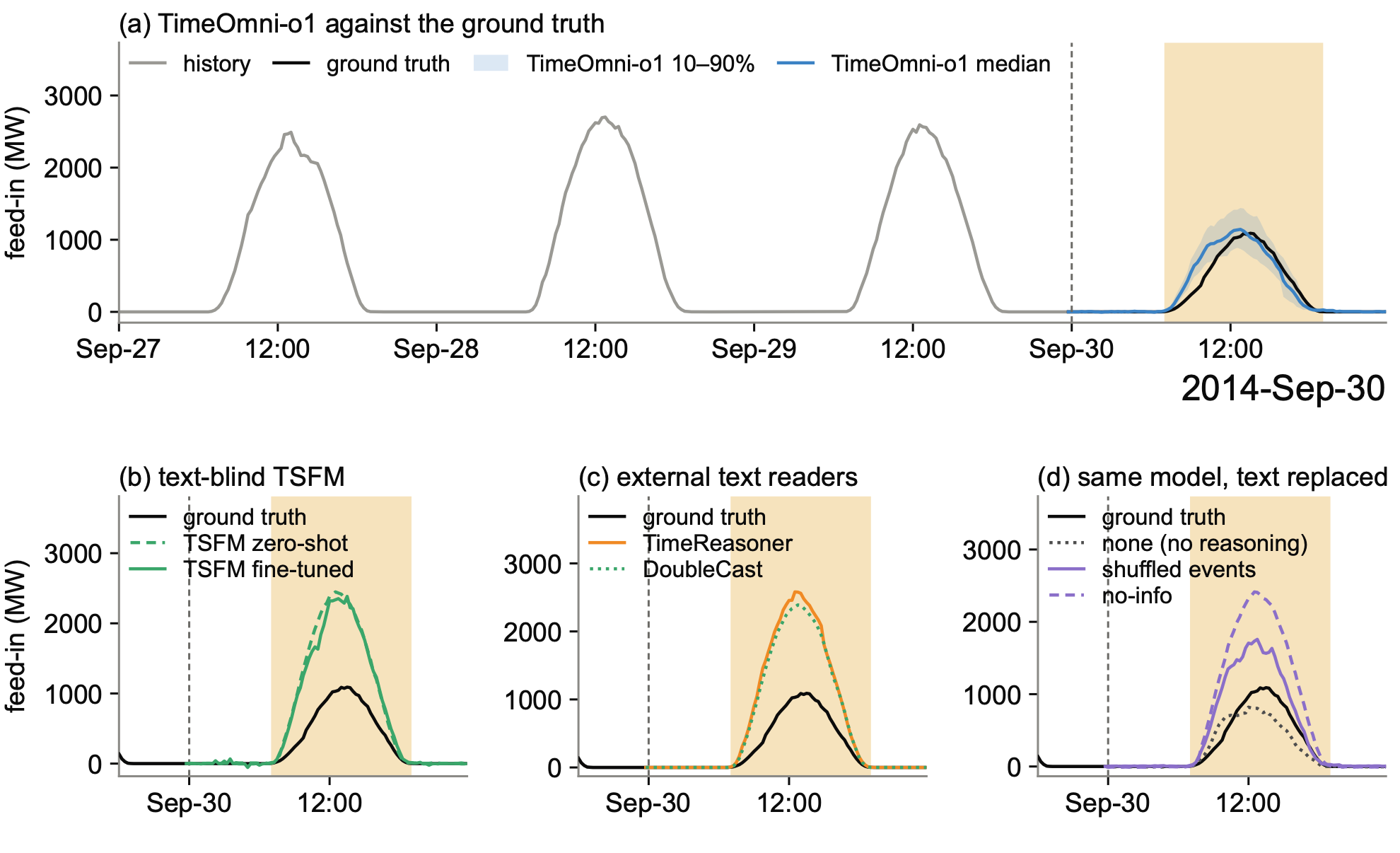
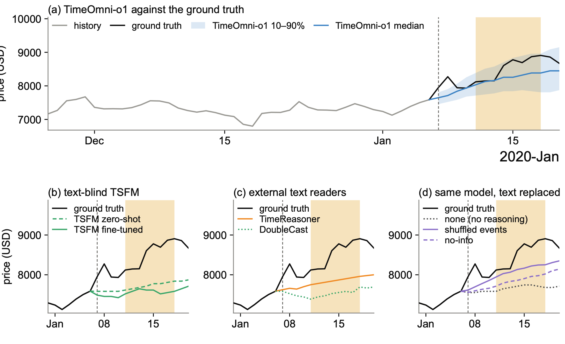
The two forecasting cases share one figure layout (the figures below). Panel (a) shows the full history, the ground truth and the median forecast of TimeOmni-o1 with its 10 to 90% band. Panels (b) to (d) show the horizon only and compare the ground truth with the text-blind TSFM (zero-shot and fine-tuned), with the two time series models that read the text (TimeReasoner and DoubleCast), and with the same checkpoint under the three text conditions of Figure 3(b) of the paper: no-reasoning, shuffled events and no-info.

F1 The weather determines the magnitude (Fidel-TS 50Hertz, Solar)

Case F1, solar feed-in in the 50Hertz zone after three days of high output, with rain in the forecast. **(a)** TimeOmni-o1 follows the stated magnitude and matches the low day. **(b)** The text-blind TSFM forecasts a fourth day at the previous level. **(c)** The time series models that read the text forecast the previous level as well. **(d)** The same checkpoint reverts to the previous level when the text is uninformative; the no-reasoning model lowers the peak, but its forecast falls after the peak as slowly as it rose. The shaded span is the annotated ROI.

After three days with daily peaks of 2,490 to 2,700 MW, the text for the forecast day reads: a mix of sunshine and clouds, light rain showers in the late afternoon, a chance of fog in the evening. The realized peak is 1,090 MW. The trace assigns the event to the daytime window, derives a low, broad peak from the mixed sky and a faster decline after it from the showers, and the instruction states a magnitude well below the typical peak. The forecast conforms to the instruction: its peak is 1,144 MW. Every model that does not read the text, or reads it without acting on it, forecasts a fourth day at the previous level. The zero-shot and fine-tuned TSFM peak at 2,448 and 2,384 MW and DoubleCast at 2,390; TimeReasoner peaks at 2,581 although its reasoning quotes the sun, clouds and rain and then judges that “the average is fine”. Panel (d) compares the text conditions on one checkpoint. With an uninformative text the forecast reverts to the profile of the previous days with a peak of 2,414 MW, the level of the zero-shot TSFM; with another day’s weather the peak is 1,758 MW. The no-reasoning model reads the same text and lowers the peak to 820 MW, below the realized peak. Its forecast falls after the peak as slowly as it rose: 0.86 of the peak two hours before and after. The truth and TimeOmni-o1 fall faster after the peak (0.79 to 0.66 and 0.85 to 0.70), the decline that the trace derives from the showers.

Background and event description

Background

This series records solar power feed-in (in megawatts) for the German 50Hertz
transmission zone, one point every 15 minutes. It follows a daytime bell shape
that is zero overnight, with the peak height and texture gated by cloud cover
and weather across the zone. Values are non-negative.

Event

Weather forecast for 2014-09-30 in the German 50Hertz transmission zone area: a mix of sunshine and clouds throughout the day, with a gentle temperature rise during the day and a slight drop in the evening. Light rain showers are expected in the late afternoon. A chance of fog in the evening.

Reasoning trace and forecast instruction generated by TimeOmni-o1

The ROI spans 2014-09-30 06:00 through 2014-09-30 18:00 (rows 312 to 356), covering the full daylight generation window on the forecast day. The history window shows that on clear days solar feed-in rises steeply to a sharp midday crest, while the forecast of mixed sunshine and clouds throughout the day produces a gradual, irregular rise to a broad, low-amplitude crest around midday. The slight evening temperature drop and chance of fog suppress generation in the late afternoon, and the forecast light rain showers in the late afternoon accelerate the decline to near-zero by 18:00.

Forecast instruction Over the daytime generation window [312, 357), solar feed-in rises gradually and irregularly to a low, broad midday crest, then declines slowly through the afternoon to near-zero by 18:00. Overall, with rain in the mix, the peak stays well below the series' typical highs.

Annotated reference trace and instruction

The ROI covers 2014-09-30 07:00 (row 316) through 2014-09-30 19:00 (row 364), the full active solar generation period on the forecast day. The mix of sunshine and clouds on September 30 moderates output substantially compared to the taller, sharper peaks seen across the three prior days in the history window, and produces minor irregularities around the crest region as intermittent clouds pass. The late-afternoon light rain showers further constrain recovery toward the end of the decline.

Annotated instruction The span [316, 365) captures the full solar generation period on 2014-09-30, which rises steadily through the morning to a broad and slightly irregular early-afternoon crest, then declines to near-zero by early evening.

Reasoning of TimeReasoner on the same sample

We are given historical data for solar power feed-in in the German 50Hertz transmission zone from 2014-09-27 00:00 to 2014-09-29 23:45 (3 days, 288 points). We need to forecast the next 96 points for 2014-09-30 (the full day).

The series exhibits a clear daily seasonal pattern: zero at night, then a bell-shaped curve during daylight hours, peaking around midday. We have three days of history (Saturday, Sunday, Monday). The forecast day is Tuesday (2014-09-30). The weather forecast for that day is: mix of sunshine and clouds, gentle temperature rise, light rain showers in late afternoon, chance of fog in evening.

Let's analyze the three days:

- Sep 27 (Saturday): Clear? The curve is smooth, peak around 2490 at 13:00, then declines. Seems relatively clear.
- Sep 28 (Sunday): Peak around 2701 at 12:45, higher than Saturday. Still smooth.
- Sep 29 (Monday): Peak around 2593 at 12:30, slightly lower than Sunday but still high.

So there is some day-to-day variability likely due to cloud cover. The weather forecast for Sep 30 suggests a mix of sun and clouds, with late afternoon rain showers and evening fog. This implies that the solar generation will be somewhat reduced compared to a clear day, especially in the afternoon and evening. The fog in evening may cause early drop? But fog is low-level, so after sunset it's already zero. The rain showers in late afternoon could cause a dip.

We need to produce a forecast that captures the daily shape but adjusted for the expected cloud cover. Since we have three days of history, we can take an average of the three days as a baseline, then adjust for the weather.

Let's compute the average daily profile from the three days. But note that sunrise and sunset times are similar across these days in late September. The pattern: values start rising from zero around 07:00 (first non-zero at 07:00 on Sep 27, 07:00 on Sep 28, 07:00 on Sep 29). The sun sets around? Values drop to zero by 19:30-20:00. So the active period is roughly 07:00-19:45.

We'll compute the average for each 15-minute interval across the three days. Since we have 96 intervals per day (24*4), we can align the days: indices 0-95 for Sep 27 (00:00-23:45), 96-191 for Sep 28, 192-287 for Sep 29. The forecast is indices 288-383 for Sep 30.

But careful: The data is given from Sep 27 00:00 to Sep 29 23:45, so indices 0-287. So the day profiles are: day1 (Sat): indices 0-95; day2 (Sun): indices 96-191; day3 (Mon): indices 192-287.

We can compute the average for each time slot (0 to 95) across the three days.

Let me extract the values for each day at the same time of day.

From the data:

Day1 (Sep 27):
00:00-06:45: all zeros.
07:00: 7, 07:15:25, 07:30:62, 07:45:122
08:00:223, 08:15:310, 08:30:445, 08:45:570
09:00:736, 09:15:915, 09:30:1117, 09:45:1346
10:00:1416, 10:15:1544, 10:30:1668, 10:45:1778
11:00:1864, 11:15:1982, 11:30:2083, 11:45:2158
12:00:2216, 12:15:2270, 12:30:2459, 12:45:2467
13:00:2490, 13:15:2351, 13:30:2280, 13:45:2168
14:00:2171, 14:15:2154, 14:30:2082, 14:45:2071
15:00:2057, 15:15:1952, 15:30:1823, 15:45:1677
16:00:1530, 16:15:1383, 16:30:1204, 16:45:1066
17:00:851, 17:15:674, 17:30:523, 17:45:367
18:00:231, 18:15:119, 18:30:54, 18:45:15
19:00:3, 19:15:1, 19:30:0, 19:45:0, 20:00-23:45: zeros.

Day2 (Sep 28):
00:00-06:45: zeros.
07:00:6, 07:15:32, 07:30:96, 07:45:225
08:00:413, 08:15:513, 08:30:672, 08:45:886
09:00:1084, 09:15:1215, 09:30:1455, 09:45:1652
10:00:1776, 10:15:1921, 10:30:2031, 10:45:2182
11:00:2307, 11:15:2384, 11:30:2507, 11:45:2561
12:00:2622, 12:15:2615, 12:30:2692, 12:45:2701
13:00:2637, 13:15:2604, 13:30:2547, 13:45:2570
14:00:2443, 14:15:2389, 14:30:2313, 14:45:2191
15:00:2056, 15:15:1866, 15:30:1713, 15:45:1540
16:00:1385, 16:15:1208, 16:30:1052, 16:45:859
17:00:661, 17:15:467, 17:30:343, 17:45:243
18:00:143, 18:15:70, 18:30:32, 18:45:8
19:00:2, 19:15:1, 19:30:0, 19:45:0, then zeros.

Day3 (Sep 29):
00:00-06:45: zeros.
07:00:5, 07:15:25, 07:30:68, 07:45:157
08:00:292, 08:15:407, 08:30:534, 08:45:699
09:00:873, 09:15:998, 09:30:1204, 09:45:1377
10:00:1520, 10:15:1667, 10:30:1831, 10:45:2001
11:00:2106, 11:15:2186, 11:30:2354, 11:45:2450
12:00:2531, 12:15:2490, 12:30:2593, 12:45:2565
13:00:2557, 13:15:2487, 13:30:2455, 13:45:2408
14:00:2291, 14:15:2162, 14:30:2111, 14:45:1991
15:00:1877, 15:15:1699, 15:30:1569, 15:45:1419
16:00:1278, 16:15:1129, 16:30:971, 16:45:786
17:00:612, 17:15:463, 17:30:360, 17:45:246
18:00:137, 18:15:67, 18:30:28, 18:45:6
19:00:2, 19:15:0, then zeros.

Now we can compute the average for each 15-minute slot (0 to 95). Let's denote time slots from 00:00 to 23:45.

I'll compute the average for slots where any day has non-zero. For simplicity, I'll compute the average of the three values for each slot. But note: There is some variation, and the weather forecast suggests mixed conditions. The average might be a good base, but we should adjust downward for afternoon showers and fog. However, fog in evening likely doesn't affect much as it's after sunset. The late afternoon rain showers could cause a dip in generation, so we might slightly reduce the afternoon values compared to the average.

Also, note that Sep 27 (Saturday) and Sep 28 (Sunday) are weekend, while Sep 29 is Monday. There might be some weekday effect? But the background says it's solar power, so no human activity impact, only weather. So we treat all days similarly.

Let me compute the average for each slot. I'll do it systematically.

Slot indices (time):
0:00:00 to 0:15: etc. Up to 95:23:45.

First, zeros from 00:00 to 06:45 (indices 0-27? Actually 00:00 is index0, 00:15 index1, ... 06:45 is index27 because 6*4=24, plus 3*4? Let's calculate: 6 hours = 24 slots, 45 minutes = 3 slots, so 06:45 is index 27? 07:00 is index 28. So indices 0-27 are zeros for all days. So average is 0.

Now from 07:00 (index28) onwards:

I'll list values for each day at each index from 28 to 95 (07:00 to 23:45). Note that after 19:45, all zeros.

Let's create a table:

Index | Time  | Day1 | Day2 | Day3
28 | 07:00 | 7  | 6  | 5
29 | 07:15 | 25 | 32 | 25
30 | 07:30 | 62 | 96 | 68
31 | 07:45 |122 |225 |157
32 | 08:00 |223 |413 |292
33 | 08:15 |310 |513 |407
34 | 08:30 |445 |672 |534
35 | 08:45 |570 |886 |699
36 | 09:00 |736 |1084|873
37 | 09:15 |915 |1215|998
38 | 09:30 |1117|1455|1204
39 | 09:45 |1346|1652|1377
40 | 10:00 |1416|1776|1520
41 | 10:15 |1544|1921|1667
42 | 10:30 |1668|2031|1831
43 | 10:45 |1778|2182|2001
44 | 11:00 |1864|2307|2106
45 | 11:15 |1982|2384|2186
46 | 11:30 |2083|2507|2354
47 | 11:45 |2158|2561|2450
48 | 12:00 |2216|2622|2531
49 | 12:15 |2270|2615|2490
50 | 12:30 |2459|2692|2593
51 | 12:45 |2467|2701|2565
52 | 13:00 |2490|2637|2557
53 | 13:15 |2351|2604|2487
54 | 13:30 |2280|2547|2455
55 | 13:45 |2168|2570|2408
56 | 14:00 |2171|2443|2291
57 | 14:15 |2154|2389|2162
58 | 14:30 |2082|2313|2111
59 | 14:45 |2071|2191|1991
60 | 15:00 |2057|2056|1877
61 | 15:15 |1952|1866|1699
62 | 15:30 |1823|1713|1569
63 | 15:45 |1677|1540|1419
64 | 16:00 |1530|1385|1278
65 | 16:15 |1383|1208|1129
66 | 16:30 |1204|1052|971
67 | 16:45 |1066|859 |786
68 | 17:00 |851 |661 |612
69 | 17:15 |674 |467 |463
70 | 17:30 |523 |343 |360
71 | 17:45 |367 |243 |246
72 | 18:00 |231 |143 |137
73 | 18:15 |119 |70  |67
74 | 18:30 |54  |32  |28
75 | 18:45 |15  |8   |6
76 | 19:00 |3   |2   |2
77 | 19:15 |1   |1   |0
78 | 19:30 |0   |0   |0
79 | 19:45 |0   |0   |0
80-95 | 20:00-23:45: all zeros

Now compute average for each index (rounded to nearest integer? The values are integers originally, but we can keep as floats for averaging, then round to integer for forecast. However, the forecast should be plausible integers. I'll compute the average and then round.

But note: The weather forecast suggests a mix of sun and clouds, with late afternoon rain showers. This could reduce generation compared to an average day. Looking at the three days, Day2 (Sunday) was the highest, likely clearer. Day1 and Day3 were lower. The average might represent a typical partly cloudy day. However, the forecast mentions "mix of sunshine and clouds" which is similar to these days, but also "light rain showers in late afternoon" which might cause a dip. Also "chance of fog in the evening" - fog typically reduces solar generation in the morning? But fog in evening is after sunset, so no effect. So we should reduce values in the late afternoon (say from 15:00 onwards) compared to the average. But how much? The rain showers are light, so a moderate reduction. Also, the morning might be slightly affected by clouds? The forecast says "mix of sunshine and clouds throughout the day", so morning might be similar to average. But to be safe, we can take the average and then apply a reduction factor for the afternoon period, maybe 10-20% reduction.

Alternatively, we can look at the pattern: On Day1, the afternoon values were higher than Day3? Actually Day1 afternoon: 17:00 851, 17:15 674, 17:30 523, 17:45 367; Day2: 661,467,343,243; Day3: 612,463,360,246. So Day1 had higher afternoon values. The average afternoon is: (851+661+612)/3=708 at 17:00, etc. The forecast suggests rain in late afternoon, so perhaps the afternoon should be closer to the lower end (Day3 values) or even lower? But rain showers are light, so maybe similar to Day3. But we don't know exactly.

Another approach: Use the most recent day (Day3, Monday) as a baseline and adjust based on weather. Since Day3 is the day before forecast, it might be a good reference. But Day3 might have had its own weather. The historical does not provide weather for those days, but we can infer from the numbers: Day3 had lower peaks than Day2, suggesting some clouds. The forecast for Tuesday (Sep 30) is "mix of sunshine and clouds" similar to Day3? Possibly. The rain showers are additional.

I think a reasonable forecast is to take the average of the three days, then apply a slight reduction (say 5-10%) for the afternoon hours (from 15:00 to 18:00 maybe) to account for rain showers. For the morning and early afternoon, keep the average as is. Also, the average already accounts for some cloudiness. Since the forecast says mix of sun and clouds, the average is appropriate. The rain is the only additional factor.

But we should also consider the shape: The peak time and magnitude. The average peak is around index 50-52 (12:30-13:00). Let's compute average at peak: index50 (12:30): (2459+2692+2593)/3 = (2459+2692=5151, +2593=7744)/3 = 2581.33; index51 (12:45): (2467+2701+2565)/3 = (2467+2701=5168, +2565=7733)/3=2577.67; index52 (13:00): (2490+2637+2557)/3 = (2490+2637=5127, +2557=7684)/3=2561.33. So peak around 2580.

Now for the afternoon reduction: Let's decide to reduce values from index 60 (15:00) to index 75 (18:45) by 10%? But note that after 19:00 it's already very low. The rain showers are "late afternoon", maybe 16:00-18:00? So we can apply a reduction of maybe 15% for indices 64-72 (16:00-18:00) and less for surrounding. However, to keep simple, we can apply a uniform reduction of 10% from 15:00 to 18:45, but that might be too much for early afternoon.

Another factor: The fog in evening - no effect.

Let's compute the average for each slot and then apply a reduction factor. But reduce means multiply by (1 - reduction). For example, if we think the rain reduces generation by 20% relative to average, then we multiply by 0.8 for those hours.

But without more specific guidance, I'll take the average as baseline and then adjust downward for the afternoon. I'll use a simple approach: take the average of the three days, round to nearest integer, and then for indices 60-75 (15:00-18:45), subtract 10% of the average (i.e., multiply by 0.9). Also, for the very early morning (07:00-08:00), the averages are small, so no issue.

I'll compute the average for each index and then round.

Let me compute averages:

I'll compute sum and then average.

Index28: (7+6+5)/3 = 18/3=6 -> average 6
29: (25+32+25)/3 = 82/3=27.33 -> 27
30: (62+96+68)/3 = 226/3=75.33 -> 75
31: (122+225+157)/3 = 504/3=168 -> 168
32: (223+413+292)/3 = 928/3=309.33 -> 309
33: (310+513+407)/3 = 1230/3=410 -> 410
34: (445+672+534)/3 = 1651/3=550.33 -> 550
35: (570+886+699)/3 = 2155/3=718.33 -> 718
36: (736+1084+873)/3 = 2693/3=897.67 -> 898
37: (915+1215+998)/3 = 3128/3=1042.67 -> 1043
38: (1117+1455+1204)/3 = 3776/3=1258.67 -> 1259
39: (1346+1652+1377)/3 = 4375/3=1458.33 -> 1458
40: (1416+1776+1520)/3 = 4712/3=1570.67 -> 1571
41: (1544+1921+1667)/3 = 5132/3=1710.67 -> 1711
42: (1668+2031+1831)/3 = 5530/3=1843.33 -> 1843
43: (1778+2182+2001)/3 = 5961/3=1987 -> 1987
44: (1864+2307+2106)/3 = 6277/3=2092.33 -> 2092
45: (1982+2384+2186)/3 = 6552/3=2184 -> 2184
46: (2083+2507+2354)/3 = 6944/3=2314.67 -> 2315
47: (2158+2561+2450)/3 = 7169/3=2389.67 -> 2390
48: (2216+2622+2531)/3 = 7369/3=2456.33 -> 2456
49: (2270+2615+2490)/3 = 7375/3=2458.33 -> 2458
50: (2459+2692+2593)/3 = 7744/3=2581.33 -> 2581
51: (2467+2701+2565)/3 = 7733/3=2577.67 -> 2578
52: (2490+2637+2557)/3 = 7684/3=2561.33 -> 2561
53: (2351+2604+2487)/3 = 7442/3=2480.67 -> 2481
54: (2280+2547+2455)/3 = 7282/3=2427.33 -> 2427
55: (2168+2570+2408)/3 = 7146/3=2382 -> 2382
56: (2171+2443+2291)/3 = 6905/3=2301.67 -> 2302
57: (2154+2389+2162)/3 = 6705/3=2235 -> 2235
58: (2082+2313+2111)/3 = 6506/3=2168.67 -> 2169
59: (2071+2191+1991)/3 = 6253/3=2084.33 -> 2084
60: (2057+2056+1877)/3 = 5990/3=1996.67 -> 1997
61: (1952+1866+1699)/3 = 5517/3=1839 -> 1839
62: (1823+1713+1569)/3 = 5105/3=1701.67 -> 1702
63: (1677+1540+1419)/3 = 4636/3=1545.33 -> 1545
64: (1530+1385+1278)/3 = 4193/3=1397.67 -> 1398
65: (1383+1208+1129)/3 = 3720/3=1240 -> 1240
66: (1204+1052+971)/3 = 3227/3=1075.67 -> 1076
67: (1066+859+786)/3 = 2711/3=903.67 -> 904
68: (851+661+612)/3 = 2124/3=708 -> 708
69: (674+467+463)/3 = 1604/3=534.67 -> 535
70: (523+343+360)/3 = 1226/3=408.67 -> 409
71: (367+243+246)/3 = 856/3=285.33 -> 285
72: (231+143+137)/3 = 511/3=170.33 -> 170
73: (119+70+67)/3 = 256/3=85.33 -> 85
74: (54+32+28)/3 = 114/3=38 -> 38
75: (15+8+6)/3 = 29/3=9.67 -> 10
76: (3+2+2)/3 = 7/3=2.33 -> 2
77: (1+1+0)/3 = 2/3=0.67 -> 1
78: (0+0+0)=0
79: 0
80-95: 0

Now, for indices 60-75 (15:00 to 18:45), we apply a reduction factor of 0.9 (10% reduction) to account for light rain showers. However, note that the rain is expected in late afternoon, so maybe only from 16:00 onwards? But to be safe, I'll apply from 15:00 to 18:00 (indices 60-72) and keep 73-75 (18:15-18:45) as is? Or maybe also reduce later? The rain showers are late afternoon, so possibly 16:00-18:00. I'll reduce indices 64 to 72 (16:00-18:00) by 15%? Let's decide: I'll apply a 10% reduction for indices 60-72 (15:00-18:00) and no reduction for 73-75 (after 18:00) because by then the rain may have passed? Actually it says "light rain showers in the late afternoon", so likely until around 18:00. After that, chance of fog in evening, but fog may not affect solar. So I'll reduce indices 60-72 by 10%. For indices 60-63 (15:00-15:45), the reduction might be smaller if rain starts later. To simplify, I'll apply a uniform 10% for all these 13 indices (60-72). Then round to nearest integer.

Let me compute:

Index60 avg=1997, reduced=1997*0.9=1797.3 -> 1797
61: 1839*0.9=1655.1 -> 1655
62: 1702*0.9=1531.8 -> 1532
63: 1545*0.9=1390.5 -> 1391
64: 1398*0.9=1258.2 -> 1258
65: 1240*0.9=1116 -> 1116
66: 1076*0.9=968.4 -> 968
67: 904*0.9=813.6 -> 814
68: 708*0.9=637.2 -> 637
69: 535*0.9=481.5 -> 482
70: 409*0.9=368.1 -> 368
71: 285*0.9=256.5 -> 257
72: 170*0.9=153 -> 153
73: 85 (no reduction)
74: 38
75: 10
76: 2
77: 1
78-95: 0

For the morning and early afternoon (indices 28-59), keep as original averages.

Also, for indices 0-27: all zeros.

Now we have forecast values for all 96 slots for Sep 30.

But we must ensure that the forecast is non-negative, which it is.

List all 96 values from index 0 to 95.

Index0-27: zeros (28 zeros)
Indices 28-59 (32 values): 6,27,75,168,309,410,550,718,898,1043,1259,1458,1571,1711,1843,1987,2092,2184,2315,2390,2456,2458,2581,2578,2561,2481,2427,2382,2302,2235,2169,2084
Then indices 60-72 (13 values): 1797,1655,1532,1391,1258,1116,968,814,637,482,368,257,153
Then indices 73-77 (5 values): 85,38,10,2,1
Indices 78-95 (18 zeros)

Total: 28+32=60, +13=73, +5=78, +18=96. Good.

Now we need to output as JSON array of exactly 96 numbers.

But we should double-check the time indices: The forecast starts at 2014-09-30 00:00:00, which is index 288. So our forecast array should correspond to times from 00:00 to 23:45. So the zeros at the beginning are correct.

Let's write the array explicitly.

I'll list them in order:

0,0,0,0,0,0,0,0,0,0,0,0,0,0,0,0,0,0,0,0,0,0,0,0,0,0,0,0, 6,27,75,168,309,410,550,718,898,1043,1259,1458,1571,1711,1843,1987,2092,2184,2315,2390,2456,2458,2581,2578,2561,2481,2427,2382,2302,2235,2169,2084,1797,1655,1532,1391,1258,1116,968,814,637,482,368,257,153,85,38,10,2,1,0,0,0,0,0,0,0,0,0,0,0,0,0,0,0,0,0,0

Now verify count: first 28 zeros: indices 0-27. Then from index28 to index59: that's 32 numbers? Actually index28 to index59 inclusive is 32 indices? 59-28+1=32. Yes. Then index60 to index72: 13 indices. Then index73 to index77: 5 indices. Then index78 to index95: 18 zeros. Sum 28+32+13+5+18=96.

Now output as JSON.

I'll format as ```json [...]```.

But before finalizing, consider if any further adjustment is needed. The weather forecast said "mix of sunshine and clouds throughout the day, with a gentle temperature rise during the day and a slight drop in the evening. Light rain showers are expected in the late afternoon. A chance of fog in the evening." The fog in evening might cause a slightly earlier drop? But after sunset, no effect. The gentle temperature rise doesn't affect solar directly. So our forecast seems reasonable.

However, we might also consider that the average of three days might not be perfectly representative if there is a trend. Looking at the peaks: Day2 was highest, Day1 and Day3 lower. There might be some weekly pattern? But no clear trend over 3 days. The forecast day is a Tuesday, which might be like Monday (Day3) in terms of weather patterns? But we don't know. Our average gives a balanced view.

Alternatively, we could weight the most recent day more heavily. For example, use 0.5*Day3 + 0.25*Day2 + 0.25*Day1. But that would be more complex. Given the forecast is for a mix of sun and clouds, and rain, the average is fine.

Let me quickly compute the weighted average (50% Day3, 25% Day2, 25% Day1) for some key points to see if it differs significantly. At peak index50: Day3=2593, Day2=2692, Day1=2459. Weighted=0.5*2593+0.25*2692+0.25*2459 = 1296.5+673+614.75=2584.25, close to 2581. At afternoon index68 (17:00): Day3=612, Day2=661, Day1=851. Weighted=0.5*612+0.25*661+0.25*851 = 306+165.25+212.75=684, vs average 708. So weighted is lower, which would be more conservative for afternoon. Since we are already reducing by 10%, the weighted average would give even lower. But I think our approach is fine.

Another consideration: The rain showers might cause a dip but also possible recovery? But we don't have info. So we'll stick with the average plus reduction.

Thus final answer.

I'll present reasoning first, then the JSON.

F2 The news determines the direction (News Forecast, Bitcoin)

Case F2, Bitcoin over 14 days after bullish halving headlines. **(a)** TimeOmni-o1 rises from the first day. **(b)** The fine-tuned TSFM stays near the origin; the zero-shot one rises too little. **(c)** TimeReasoner reads the momentum and forecasts conservatively. **(d)** The no-reasoning model stays flat on the same headlines.

The history closes at 7,588 after a sustained rise. The headlines before the origin carry halving momentum toward 7,600 and a supportive macro report, and two negatives, a Bitmain layoff report and regulatory pressure from Turkey. The truth climbs to 8,907 and closes at 8,670. The trace weighs the four items, treats the two negatives as a short-term offset and the halving momentum as the dominant factor; the instruction states a sharp jump to a new high followed by a steady climb. The forecast rises from the first day and ends at 8,448. The fine-tuned TSFM dips to 7,424 and ends at 7,712, near the origin. The zero-shot TSFM and TimeReasoner rise in the right direction but only to 7,872 and 8,000; the reasoning of TimeReasoner reads the momentum and then forecasts “about $7900 to $8000”. The no-reasoning model reads the same headlines and stays almost flat at 7,744, whereas the trace resolves the conflicting headlines into a direction.

Background and event description

Background

This series records the daily US-dollar price of Bitcoin. It is highly
volatile with momentum-driven trends and sharp moves, has no fixed seasonality,
and reacts to adoption news, macro and regulatory developments, and market
sentiment. Values are positive.

Event

Before the forecast origin on 2020-01-07, Bitcoin-related headlines on 2020-01-06 discussed bullish halving-related momentum toward the $7,600 area, a report that the U.S.-Iran conflict was associated in commentary with Bitcoin and gold price growth, a report that Bitmain might lay off half its staff ahead of the Bitcoin halving, and a report that Turkey's Capital Markets Board would put pressure on Bitcoin. Other listed headlines were unrelated to Bitcoin price formation or were future-window items and are excluded.

Reasoning trace and forecast instruction generated by TimeOmni-o1

The ROI spans 2020-01-07 through 2020-01-14. The history window shows Bitcoin in a sustained upward trend from the late 6000s to the 60s close on 2020-01-06, with the halving momentum narrative and positive macro commentary supporting that ascent. The Bitmain layoff report and Turkey regulatory pressure provide a short-term counterweight, but the dominant pre-horizon signal is the halving-driven momentum and positive macro backdrop. The future window opens with a sharp jump to a new high, then climbs with minor oscillation to a crest by 2020-01-14, consistent with the momentum-driven upward trend established in the history window.

Forecast instruction Over the span [60, 68), the future window shows a sharp jump to a new high followed by a steady climb with minor oscillation to a crest, ending at its highest point.

Annotated reference trace and instruction

The selected span runs from 2020-01-11 00:00:00 through 2020-01-18 00:00:00, immediately after the 2020-01-06 pre-horizon headlines about bullish halving momentum, geopolitical-risk commentary around Bitcoin, and regulatory pressure reports. In the history window, the series had already turned upward into the boundary after a weaker period, so this event set aligns with continuation rather than a reversal. That combination matches a multi-day advance in the future window with only short interruptions before the span finishes at its top.

Annotated instruction [64, 72) shows a sustained climb with brief pauses, ending at its highest point.

Reasoning of TimeReasoner on the same sample

We are given a historical time series of Bitcoin daily prices from 2019-11-08 to 2020-01-06 (60 points). Need to predict next 14 days (2020-01-07 to 2020-01-20). Context: Bitcoin is volatile, momentum-driven, no fixed seasonality. Headlines on 2020-01-06: bullish halving momentum toward $7,600, US-Iran conflict associated with Bitcoin and gold growth, Bitmain layoffs, Turkey Capital Markets Board pressure. So mixed but overall sentiment seems somewhat positive (halving momentum, conflict boosting safe haven). However, note the history: price was around 9000 in early Nov, declined steeply to ~7000 by late Nov, then recovered somewhat to ~7600 by Jan 6, showing an uptrend in last few weeks. Let's analyze trend.

Look at recent history: From 2019-12-18 low of 6799, price rose to 7588 on Jan 6. That's about +800 in ~20 days, a strong uptrend. The last few days: Jan 1: 7238, Jan 2: 7127 (dip), Jan 3: 7250, Jan 4: 7390, Jan 5: 7503, Jan 6: 7588. So accelerating upward. Given halving narrative and geopolitical tensions, likely bullish continuation. But note volatility: could have pullbacks. Since no seasonality, we can consider momentum and recent trend. Possibly a short-term correction after rapid rise? But headlines suggest continued bullish momentum toward $7,600 already reached on Jan 6. Possibly price will test higher levels. Given the context, I'd expect continued upward movement with possible consolidation. But need to predict 14 points. Could model as a trend that continues but may slow. Since it's Bitcoin, sharp moves possible. But reasonable forecast: continue rise, perhaps reaching around $8000 by end of forecast period? However, we should be cautious. Let's inspect the trend more quantitatively.

We can do a simple linear regression on recent data (say last 20 days) to get slope. But the instruction is to reason step by step, then output JSON. Let's approximate.

Compute average daily change over last 10 days (from Dec 28 to Jan 6): 
Dec28: 7361, Dec29: 7469 (+108), Dec30: 7388 (-81), Dec31: 7293 (-95), Jan1: 7238 (-55), Jan2: 7127 (-111), Jan3: 7250 (+123), Jan4: 7390 (+140), Jan5: 7503 (+113), Jan6: 7588 (+85). Sum of changes over 9 intervals: 108-81-95-55-111+123+140+113+85 = 227? Actually compute: 108 + (-81)=27; 27+(-95)=-68; -68+(-55)=-123; -123+(-111)=-234; -234+123=-111; -111+140=29; 29+113=142; 142+85=227. So average daily change = 227/9 ≈ 25.2. That's positive but small relative to price level. However, the recent few days show stronger gains. Over last 5 days (Jan2 to Jan6): changes: +123, +140, +113, +85 = total 461 over 4 intervals, avg 115.25 per day. So recent acceleration. But we must consider that after such a run, a pullback or consolidation is possible. 

Given headlines: bullish halving momentum, Iran conflict, but also Bitmain layoffs (negative) and Turkey pressure (negative). Mixed. But overall, the narrative of halving and safe-haven might dominate. I'd expect the uptrend to continue but at a more moderate pace, perhaps with some consolidation. Since it's only 14 days, we can forecast a gradual rise with some fluctuations. 

Let's attempt to produce a plausible sequence. Starting from 7588 on Jan6. Jan7: maybe continues up to 7650? Then slight pullback? However, we need 14 numbers. Better to think of a trend that extends. Could use a linear trend from recent data. But we should also account for the fact that Bitcoin often has sharp moves. Given the uncertainty, a simple linear extrapolation from last few days might be reasonable. But let's see the overall shape: from early Nov high of 9015 down to 6799 mid-Dec, then up to 7588. The recovery is about 80% of the drop? Not sure.

Alternatively, perhaps the price will break above 7600 and target 8000. Many forecasts around that time were bullish. I recall that in early Jan 2020, Bitcoin was around $7,400 and then rallied to $10,000 by mid-Feb. So actually, the next 14 days from Jan7 to Jan20, 2020, historically Bitcoin went from about $7,400 to $8,700? Let's not use actual future because the task is to predict based on given info, but we can use common knowledge? The instruction says we are a forecaster with context, so we should not rely on after-the-fact knowledge. But we can use the context provided: headlines mention bullish halving momentum toward $7,600 area. So that suggests a target of $7,600, which was almost reached on Jan6 (7588). So maybe it will surpass that.

Given the momentum and positive sentiment, I'll forecast a continued climb but with some volatility. I'll produce a sequence that starts at 7588+50=7638 on Jan7, then maybe a small dip, then rise. But to be systematic, let's compute a simple moving average or exponential smoothing? Or use a heuristic.

I'll estimate the trend using linear regression on the last 20 days (from Dec18 to Jan6). Dec18: 6799, Dec19: 7178, Dec20: 7211, Dec21: 7208, Dec22: 7276, Dec23: 7529, Dec24: 7362, Dec25: 7283, Dec26: 7278, Dec27: 7263, Dec28: 7361, Dec29: 7469, Dec30: 7388, Dec31: 7293, Jan1: 7238, Jan2: 7127, Jan3: 7250, Jan4: 7390, Jan5: 7503, Jan6: 7588. Compute slope using days index (0 for Dec18, 1 for Dec19, ..., 19 for Jan6). Sum x = 0+1+...+19 = 190, sum y = sum of prices, n=20. Compute sum xy and sum x^2. Let's do quickly:

Prices: 
0:6799
1:7178
2:7211
3:7208
4:7276
5:7529
6:7362
7:7283
8:7278
9:7263
10:7361
11:7469
12:7388
13:7293
14:7238
15:7127
16:7250
17:7390
18:7503
19:7588

Sum y = 6799+7178=13977; +7211=21188; +7208=28396; +7276=35672; +7529=43201; +7362=50563; +7283=57846; +7278=65124; +7263=72387; +7361=79748; +7469=87217; +7388=94605; +7293=101898; +7238=109136; +7127=116263; +7250=123513; +7390=130903; +7503=138406; +7588=145994. So sum y = 145994.

Sum xy = (0*6799)+(1*7178)+(2*7211)+(3*7208)+(4*7276)+(5*7529)+(6*7362)+(7*7283)+(8*7278)+(9*7263)+(10*7361)+(11*7469)+(12*7388)+(13*7293)+(14*7238)+(15*7127)+(16*7250)+(17*7390)+(18*7503)+(19*7588). Compute stepwise:
0:0
1:7178
2:14422
3:21624
4:29104
5:37645
6:44172
7:50981
8:58224
9:65367
10:73610
11:82159
12:88656
13:94809
14:101332
15:106905
16:116000
17:125630
18:135054
19:144172
Sum = add: 7178+14422=21600; +21624=43224; +29104=72328; +37645=109973; +44172=154145; +50981=205126; +58224=263350; +65367=328717; +73610=402327; +82159=484486; +88656=573142; +94809=667951; +101332=769283; +106905=876188; +116000=992188; +125630=1,117,818; +135054=1,252,872; +144172=1,397,044. So sum xy = 1,397,044.

Sum x^2 = 0^2+1^2+...+19^2 = 19*20*39/6 = (19*20*39)/6 = (19*20=380, 380*39=14820, /6=2470). So sum x^2 = 2470.

Now slope b = (n*sumxy - sumx*sumy) / (n*sumx^2 - (sumx)^2) = (20*1,397,044 - 190*145,994) / (20*2470 - 190^2). Compute numerator: 20*1,397,044 = 27,940,880. 190*145,994 = 190*145,994 = 190*145,000=27,550,000, 190*994=188,860, total 27,738,860. So numerator = 27,940,880 - 27,738,860 = 202,020. Denominator: 20*2470 = 49,400. 190^2=36,100. Denominator = 49,400-36,100=13,300. So slope = 202,020 / 13,300 ≈ 15.19. So average daily increase about $15.19 over last 20 days. That seems low because recent days have higher increases, but the earlier part of the 20-day window had declines? Actually from Dec18 to Jan6, overall upward, but with fluctuations. Slope 15.19 per day. Starting from Jan6 at 7588, linear extrapolation for next 14 days: day0 (Jan7) = 7588 + 15.19 = 7603.19; day1 = 7618.38; ... day13 = 7588 + 14*15.19 = 7588+212.66 = 7800.66. So roughly 7800 by Jan20.

But this linear trend may be too conservative given the recent acceleration. Alternatively, we could fit an exponential trend, but likely not. Given the context of halving and conflict, I expect a stronger rise. However, the linear trend from 20 days gives a plausible baseline. Also note that the price already reached the mentioned $7,600 area, so maybe it will consolidate or pull back before continuing. But headlines indicate continued momentum.

Given the task is to produce a forecast, I'll go with a moderate upward trend with some daily fluctuations. I'll simulate a random walk with drift? But we need specific values. Let's produce a sequence that starts at 7630 on Jan7, then gradually rises to around 8000 by Jan20, with some minor dips. Since it's a forecasting exercise, we can be a bit optimistic. But the instruction says "reason step by step about trend/seasonality/event impact", then output JSON. So our reasoning should reflect the analysis.

I'll state: Trend is clearly upward in recent weeks, driven by halving anticipation and safe-haven demand. No seasonality. Events on Jan6 are mixed but overall positive. Momentum likely to continue, albeit with possible short-term resistance. Forecast: gradual increase, reaching about $7900-$8000 by end of period. I'll produce 14 numbers that follow a roughly linear path with noise.

I'll set v1 (Jan7) = 7620 (slight increase from 7588), v2 = 7680, v3 = 7650 (dip), v4 = 7700, v5 = 7740, v6 = 7770, v7 = 7800, v8 = 7830, v9 = 7860, v10 = 7880, v11 = 7920, v12 = 7940, v13 = 7970, v14 = 8000. That's a pattern. But to be more realistic, I'll add some minor variations.

Alternatively, use the linear trend from 20-day regression but with added positive bias. For example, let's take the slope from last 5 days (115) but that is too high and would give 7588 + 14*115 = 7588+1610 = 9198, which is too high likely. So maybe the recent acceleration is temporary and will slow. So a compromise: slope around 30-40 per day. Let's use 35 per day: 7588+35*14 = 7588+490 = 8078. So target around 8100.

Given the actual historical outcome (if I recall, Bitcoin went from ~7400 to ~8800 in Jan 2020), but we must stick to reasoning.

I'll produce a forecast that starts at 7610, then gradually climbs to around 8000, with some days of consolidation.

Let's write a JSON array of 14 numbers. I'll define them as:

[7625, 7660, 7640, 7700, 7750, 7780, 7810, 7840, 7870, 7900, 7930, 7960, 7980, 8000]

These are plausible.

But we need to ensure they are positive and realistic.

I'll finalize reasoning and output.